Notice:
This post is older than 5 years – the content might be outdated.
There has always been a gap between the capabilities of men and machine. While computers were able to perform complex multiplications or store large amounts of data, humans beat them on rather intuitive tasks like natural language or perception. The research area of Artificial Intelligence (AI) aims to bridge this gap by bringing consciousness and genuine intelligence into machines and programs. Recent developments in a subfield of AI promise to reduce the existing gap. This subfield of AI is called Deep Learning (DL) and its impact reaches out to different domains of application, like computer vision or machine translation.
Just imagine a little robot rephrasing one of the most famous sentences in human history, just because he got a software update that included DL:
That’s one small step for [a] man … one … giant leap for AI.
This blogpost provides an overview on DL and discusses how it fits into the framework of AI. Thereby it will serve as an introduction into the topic and a reference point for more advanced contributions in this blog. For this purpose, we will answer the following questions:
- What makes up learning for a computer program?
- How are Artificial Intelligence and Deep Learning related?
- What are the building blocks of Deep Learning?
- Why is all of this happening right now?
- Where are we going next?
How do Computer Programs Learn?
In order to gain a first intuition of computer programs that learn, we will have a look at a definition provided by Tom Mitchell [1]:
A computer program is said to learn from experience E with respect to some class of tasks T and performance measure P, if its performance at tasks in T, as measured by P, improves with experience E.
According to this definition, learning comprises three components. First of all, learning is always assessed in connection to a specific task T. Henceforth, we will use the example of a simple classification task to support our explanations. Let’s assume we have a large stack of images that either show a single dog or a cat. We are interested in building a model that is able to assign one of these two classes at the moment we show it a specific picture. In other words, our task T is defined as a classification problem with two classes („cat“ and „dog“).
Furthermore, we want to evaluate our model based on its performance P. Typically, one relies on quantitative metrics to specify the performance of a model. In our case, we want the model to label as many images as possible with the correct class. Therefore, we will use a metric called accuracy. This metric measures the share of correct classifications over all processed samples. Let’s stick with our example and suppose we have a set of 1000 images (500 „cat“ and 500 „dogs“). Since our model is not perfect yet, it will confuse some cats with dogs and some dogs with cats. E.g., our model gets 540 out of the labels correctly (correct „cats“: 300, correct „dogs“: 240). This corresponds to an accuracy of 54% (share of correct classifications).
The third component that matters for computer programs that learn is experience E. In order to stimulate a learning process we provide a dataset to our model. In our example the dataset consists of our image stack (1000 images) annotated with the corresponding ground truth labels („cat“, „dog“). For training purposes, we let our model predict the class for a certain image and compare the prediction to the ground truth. Based on this comparison we provide a feedback (loss) to our model, which uses it to adjust its parameters. Thereby, our model aims to improve its predictive behaviour for future predictions based on similar inputs. In other words: the more images our model has seen, the more experience it gains and the better it becomes at recognising cats and dogs.
So far, we have introduced what it means for a computer program to learn. In a next step, we will discuss different concepts that incorporate learning and show their relations within the field of Artificial Intelligence.
How are Artificial Intelligence and Deep Learning Related?
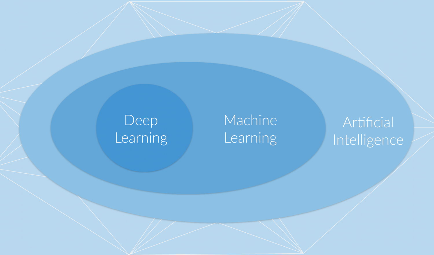
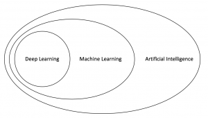
There are two important frameworks that incorporate computer programs that learn, namely Machine Learning (ML) and DL. In order to understand the relation between those concepts and AI, one should have a basic understanding of Artificial Neural Networks (ANNs). Below we present brief explanations of the different concepts.
- Artificial Intelligence: deals with intelligent agents, which perceive their environment and derive actions in order to maximise chances to accomplish a certain goal.
- Machine Learning: describes computer programs that learn to solve tasks (e.g. distinguish between two classes based on a set of features) without being explicitly programmed.
- Deep Learning: algorithms learn to solve tasks by exploring the latent structure of the data with the help of ANNs that have several hidden layers.
On the first glance, it appears that these definitions are very similar. Indeed, there is an overlap between the different concepts as shown in the following figure and which will be discussed now.
Artificial Intelligence
Our intuitive expectation of Artificial Intelligence is mainly shaped by our experience with natural intelligence. We expect a machine with human-like cognitive capabilities. In this regard, the machine should e.g. act smart, plan in advance, learn and be creative. If we combine the formal explanations of the previous section and this initial expectation, we end up with an agent (a physical machine or a program) that adjusts its behaviour towards a goal based on observations about its environment.
Apple’s digital assistant Siri is designed to carry out tasks through interaction with humans. As long as the focus of a task is to schedule calendar entries or retrieve the weather forecast, there is no clue that Siri is a program. Although, I guess every iPhone owner successfully tried to push Siri beyond its limits. These little experiments show that the system is neither conscious nor genuinely intelligent. Hence, Siri can be described with the concept of weak or narrow AI. Instead of investigating the reasoning process behind actions, the observed behaviour itself is assessed. This allows us to attribute intelligence to agents that are applied in narrow domains and with limited focus. The term of narrow AI is particularly interesting within business context, since it can be used to summarise all kinds of automated decision making tools.
Strong or general AI goes beyond automated decision making and is concerned about machines that actually think. Thereby it is a closer match to our initial expectation based on natural intelligence. A key capability of strong AI is to transfer acquired knowledge in order to perform on more general tasks and adapt to new problems.
A Narrow AI Based on a Set of Rules
With this in mind, we will draft a narrow AI that allows us to classify our image stack. At this point, we will make a naive assumption about the world of cats and dogs. We suppose that we can distinguish them based on two features only, their snouts and their tails. While cats tend to have flat snouts as well as long but thin tails, the appearance of dogs is more diverse.
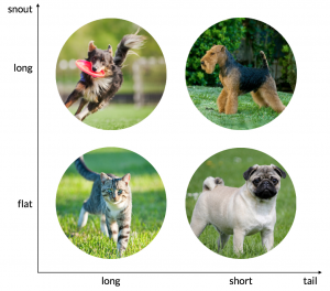
In order to perform a classification, we need to extract those two features from the raw pixels of the images. For now, we will rely on a blackbox pre-processing step that provides us with the features form_of_snout and form_of_tail. This pre-processing step is performed by an external component, which is not part of our classifier. This assumption represents a drastic simplification of the real problem, but it allows us to formulate our narrow AI by the following rules:
|
1 2 3 4 5 6 7 |
if form_of_snout == 'flat' and form_of_tail == 'long': label = 'cat' else: label = 'dog' |
As soon as we aim for a more realistic version of our use case the complexity of our model increases. In order to improve our AI, it would require more rules and more features. We would need to make sure that every exception (e.g. dogs with flat snouts and long-thin tails) is captured by a corresponding rule. As one can imagine, we would spend a vast amount of time formulating these rules and end up with a large system. However, the resulting system would have almost no flexibility and the occurrence of unknown examples would require us to re-write the code.
Machine Learning
Machine Learning is a subset of AI that overcomes this limitation of rule-based AI systems. Instead of using a set of pre-defined rigid rules, ML algorithms learn to find patterns in the data based on previous observations. In other words, we assume that there is a (more or less complex) function which explains the data and ML algorithms infer decision rules that approach this function. Learning from experience means nothing else than adjusting these decision rules over time.
The power of ML comes from the fact that algorithms learn from the data passed to them. Thereby, they can be re-used without being re-written. If we collect another dataset that captures the distinction between elephants and giraffes, we could train a similar type of classifier as we used for our cat-dog classification problem. Due to their design, the power of ML algorithms heavily depends on quality of the input data. Algorithms cannot predict what they have not seen before. E.g. without re-training, our cat-dog classifier would assign either „cat“ or „dog“ to an image that shows an elephant.
A (Shallow) ML-based Approach
As we did for our rule-based AI, we will stick to our assumption of how one can distinguish between cats and dogs. Furthermore, we rely on the same blackbox pre-processing tool which extracts the features from our images. Based on the extracted features we could then apply standard ML algorithms like Decision Trees, Logistic Regression or Support Vector Machines to classify samples from our dataset.
The illustration below gives you an intuition how ML algorithms learn. Let’s say we decided to use a model allowing us to split our data linearly. After seeing some samples, the algorithm detects a relation between the snout of the animal and its class. Therefore, the model will predict „dog“ for images where the feature form_of_snout is long and „cat“ if is flat.
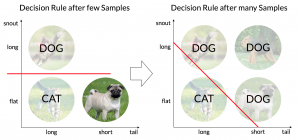
At some point in time, our model needs to classify the image of a pug. As one can see, pugs do have a flat snout but belong to the class „dog“. Hence, there is a mismatch between the prediction of the model and the ground truth of the image. This mismatch is quantified by a loss function and fed back into the model. Based on this feedback, the model adjusts its parameters (changes intersection and slope of the decision rule). Over time, the model’s decision rule approaches the latent function that explains the data.
Deep Learning
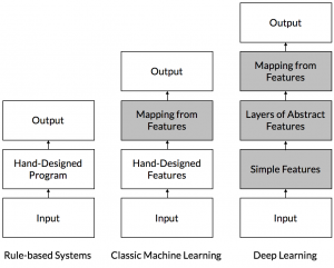
So far, we showed the advantage of learnable models over programs that make use of rigid rules. Nevertheless, rule-based models as well as shallow ML algorithms rely on pre-processing in order to extract features like form_of_snout from the images. Instead of relying on feature engineering, DL leverages artificial neural networks to learn the features itself (also known as representation learning) and build feature hierarchies from it.
A Deep Cat-Dog Classifier
Using artificial neural networks to build our classifier allows us to process raw images instead of engineered features. In our case, we feed the raw pixels of an image (i.e. its numeric representation: RGB-value) into the input layer. Neurons of the first layer typically respond to simple shapes such as edges or straight lines. These features are then used to detect more complex structures within the higher layers of the network. There might be neurons that respond to a dogs snout, a cats tail or a dogs chest. In the top layer of the network, activations of higher level neurons are combined in order to predict the most likely class of the image.
Let’s compare this to what we have learned about ML in general. Shallow ML models learn to make predictions based on a set of features that obtained by an additional pre-processing step. In contrast, deep neural networks do also learn to capture characteristics of the data that are important to solve a task.
What makes up Deep Learning? — The Building Blocks
Deep Learning builds on Artificial Neural Networks (ANNs) which mimic the behaviour of the human brain. First attempts to simplify and formally describe the way human brains work date back to the 1950’s and 1960’s. In this blog post you will find an introduction into ANNs in general. Recent developments in the field of Deep Learning are based on more advanced neural architectures. Subsequently, we will summarise two families of networks that deviate from standard feedforward networks.
Convolutional Neural Networks (CNNs)
The idea behind CNNs is to make use of grid-like inputs, e.g. images. They were introduced in 1980 by Fukushima [4] and firstly deployed by LeCun et al. in 1989 [5]. CNNs resolve two limitations of feedforward networks. Firstly, CNNs drop the concept of fully connected layers and thus reduce the amount of weighted connections in the network. Thereby, training a model requires less time due to fewer adjustable parameters. Furthermore, it allows to train CNNs in a highly parallel manner. Secondly, pixels in an image turn out to be highly related to pixels of their neighbourhood. Unlike fully connected networks, CNNs make use of the neighbourhood of pixels to capture these dependencies.
CNNs drew attention due to their success in the ImageNet challenge in 2012. Alex Krizhevsky won the challenge with his CNN called AlexNet and outperformed all of the competing models by far [6]. Since then, CNNs have been the most favourable neural architecture when it comes to image recognition. AlexNet consisted of eight layers with about 500’000 neurons and 60 million trainable parameters. Five of its layers were so called convolutional layers and three were fully connected ones. Some of the convolutional layers were followed by pooling layers. As one can imagine, AlexNets complexity goes way beyond something that we can achieve with systems we discussed before (rule-based and shallow ML).

Recurrent Neural Networks (RNNs)
Sequential data is characterised by the dependencies between different elements of the sequence. Let’s consider a tangible example: natural language is nothing else than a sequence of words. If we use the word „bank“ in the same sentence with „money“ it will have a another meaning than within a sentence that contains „sitting“. In other words, the meaning „bank“ depends words that were used prior to it.
Since feedforward networks treat their input independently, they are not able to grasp these nuances. RNNs overcome this limitation due to cyclic connections. These connections incorporate a memory capability and enable RNNs to capture temporal dependencies within the data. Hence, RNNs have been successfully applied to tasks like speech recognition, time series prediction and gesture recognition.
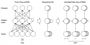
Above a simple example of a RNN is shown. As you can see on the left side, the neural network consists of three layers. The network has an input layer that consists of five neurons and an output layer that consists of three neurons. Input and output layer are connected through a single hidden layer with three neurons in it.
All neurons of the hidden layer have cyclic (recurrent) connections to themselves. Their meaning becomes more clear if we add time as a dimension into our consideration. A look on the right side reveals that the neurons in the hidden layer at t do not only depend on the input layer at t. In addition, they receive the state of the neurons in the hidden layer at t-1. Both inputs are concatenated and processed by a non-linear activation function. The resulting hidden state is then used to compute the output at t and to update the hidden layer at t+1.
Machine Translation with RNNs
A popular example that uses RNNs is machine translation. In 2016, Google announced that their Neural Machine Translation (NMT) improved the state-of-the-art and approached human performance [7].

Afterwards, the decoder RNN predicts a sequence of words (now in English) based on this summary and its previous predictions. E.g. at \(d_2\), the decoder knows about the context of the input and is aware that it already predicted: „Knowledge is“. Hence, it predicts that „power“ as the token with the highest probability to continue that sequence. When the decoder predicts the end-of-sequence symbol <end>, the decoder terminates and the produced sequence is presented to the user.
Advanced RNNs: Long-Short Term Memory networks (LSTMs)
In practice, standard RNNs have difficulties to capture long-term dependencies. LSTMs are an RNN-architecture designed to overcome this limitation due to the use of connecting weights which work as gates. In particular, those gates enable the LSTM to decide whether it should keep old information or update its memory with new information. When compared to standard RNNs, LSTMs show better performance especially on longer sequences. Due to this advantage LSTMs gained popularity and have been applied in a variety of tasks. This blogpost gives a well written introduction into LSTMs that will help you to gain compelling insights.
Why is Deep Learning happening right now?
The underlying concepts of artificial neural networks are not new. Already in 1958, Rosenberg proposed the Perceptron, which is the predecessor of today’s ANNs. Even more advanced architectures like CNNs (1980) or LSTMs (1997) date back before the millennium. But if the recent hype about DL and AI is not due to new disruptive models, why is it happening right now?
Availability of large-scale datasets
In order to answer this question, one needs to take a glance on tasks that have been solved with the help of DL. AlexNets breakthrough in computer vision was based on about 1.2 million training images from the ILSVRC (Imagenet Large Scale Visual Recognition Competition). Another example is Stanford’s pre-trained GloVe model [8]. In order to retrieve vector representations for words (embeddings), they trained their model on different corpora that consisted of billions of tokens and millions of distinct words. These are only two of many examples where DL models developed their full potential in the presence of large-scale datasets and thereby helped to solve challenging tasks.
A large share of our life happens to be digital. We order online via Amazon. We communicate via What’s App or Facebook. We share our knowledge in platforms like Wikipedia. We translate via Google Translate or DeepL. Already for our private life, this seems to be a never ending story. This story grows even more if we take companies and their daily business into account. Since life moved from the analogous world to the digital one, it is easier to collect and create large-scale datasets. The availability of these datasets is one of the main reasons that cause the current hype around DL and AI.
Ian Goodfellow refers to the following rule of thumb [2]: for a classification task it requires about 5,000 labeled examples to achieve a acceptable performance. A model trained on a dataset with at least 10 million labeled examples will match or exceed human performance.
Reduced training times due to an improved infrastructure
Another important development are improvements within the infrastructure that is required to perform DL experiments. On a first glance one would fully attribute this to more available computational power. Indeed, this is a very important fact. Faster CPUs and the integration of GPUs into the training process significantly reduced training times. In case of the GPUs this was achieved by a massive parallelisation of computations.
Additionally, progress have been made due to advances in the software infrastructure. Publicly available libraries like Tensorflow, Keras, Pytorch and others represent interfaces with a pleasant level of abstraction. Thereby, it becomes easier for developers to build and deploy DL models. Furthermore, entry barriers for beginners shrink. The resulting demand for education is covered by an endless amount of online tutorials and courses across many platforms.
Advances in training ANNs
Eventually, we should not fully ignore the underlying models. While the different ANN-architectures do have a few years on their hump, there have been advances in the way of training them. Since 2006, the general interest in ANNs increased after Geoffrey Hinton presented an efficient strategy to pre-train deep belief nets [9]. Later work applied these insights to other kind of deep neural networks.
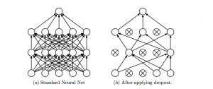
Furthermore, there have been advances that improved certain characteristics of ANNs in general. For instance, the introduction of a method called dropout allows ANNs to switch off some of their neurons during computation. Since the corresponding information now needs to be captured by other neurons, dropout increases the generalisation of the respective ANN [10].

What’s next?
In 2016, Google’s subsidiary DeepMind developed a program called AlphaGo and challenged the world champion in Go, Lee Sedol. Tech enthusiasts and members of the Go community all over the world were watching when AlphaGo defeated Lee Sedol in four out of five matches. This is astonishing since Go is a board game comparable to chess, but with way higher complexity. Shortly thereafter, Demis Hassabis (founder of DeepMind) draw an interesting conclusion about the impact of AlphaGo.
Lee Sedol has won every single game he has played since the #AlphaGo match inc. using some new AG-like strategies – truly inspiring to see!
— Demis Hassabis (@demishassabis) 5. Mai 2016
From his point a view, Lee Sedol was able to improve his performance as a professional by learning from AI. Hassabis‘ statement is evidence of a mindset that points into a future where AI augments our world instead of being an apocalyptic threat.
Our experience with Deep Learning
The list below provides an overview on our hands-on experience with DL. Don’t worry, have a closer look to get an intuition of what is possible.
- Text Spotting using semi-supervised Generative Adversarial Networks
- Machine Learning as a Service
- From Exploration to Production — Bridging the Deployment Gap for Deep Learning, (2)
- Generative Adversarial Networks explained
- Dark Side of AI/ML
References
- [1] Mitchell, T. M. (1997). Machine learning. WCB.
- [2] Goodfellow, I., Bengio, Y., Courville, A., & Bengio, Y. (2016). Deep learning (Vol. 1). Cambridge: MIT press.
- [3] Explanation of Universal Function Approximation:
- [4] Fukushima, K. (1988). Neocognitron: A hierarchical neural network capable of visual pattern recognition. Neural networks, 1(2), 119-130.
- [5] LeCun, Y., Boser, B., Denker, J. S., Henderson, D., Howard, R. E., Hubbard, W., & Jackel, L. D. (1989). Backpropagation applied to handwritten zip code recognition. Neural computation, 1(4), 541-551.
- [6] Krizhevsky, A., Sutskever, I., & Hinton, G. E. (2012). Imagenet classification with deep convolutional neural networks. In Advances in neural information processing systems (pp. 1097-1105).
- [7] GNMT Google 2016: Link
- [8] Pennington, J., Socher, R., & Manning, C. (2014). Glove: Global vectors for word representation. In Proceedings of the 2014 conference on empirical methods in natural language processing (EMNLP) (pp. 1532-1543).
- [9] Hinton, G. E., Osindero, S., & Teh, Y. W. (2006). A fast learning algorithm for deep belief nets. Neural computation, 18(7), 1527-1554.
- [10] Srivastava, N., Hinton, G., Krizhevsky, A., Sutskever, I., & Salakhutdinov, R. (2014). Dropout: a simple way to prevent neural networks from overfitting. The Journal of Machine Learning Research, 15(1), 1929-1958.
- [11] Bahdanau, D., Cho, K., & Bengio, Y. (2014). Neural machine translation by jointly learning to align and translate. arXiv preprint arXiv:1409.0473.