Notice:
This post is older than 5 years – the content might be outdated.
Neural networks are one of the technologies that have the potential to change our lives forever. Besides lots of applications and machines in the industry they have disrupted the domain of image and text generation as well as machine translation with the deployment of Generative Adversarial Networks (GAN). Furthermore recent improvements on the architecture and the training of GAN have rendered them even applicable on a greater variety of problems, e.g sequential or discrete data. In this blog article we want to take a closer look on the general theoretical GAN architecture and its variations.
First of all GAN are a type of model that employs neural networks. If you are not yet familiar with the basic notions of a neural network, you can find a nice introduction in the free material provided by Michael Nielsen. A more comprehensive and detailed discussion can be found here.
The Basic Idea of Generative Adversarial Networks
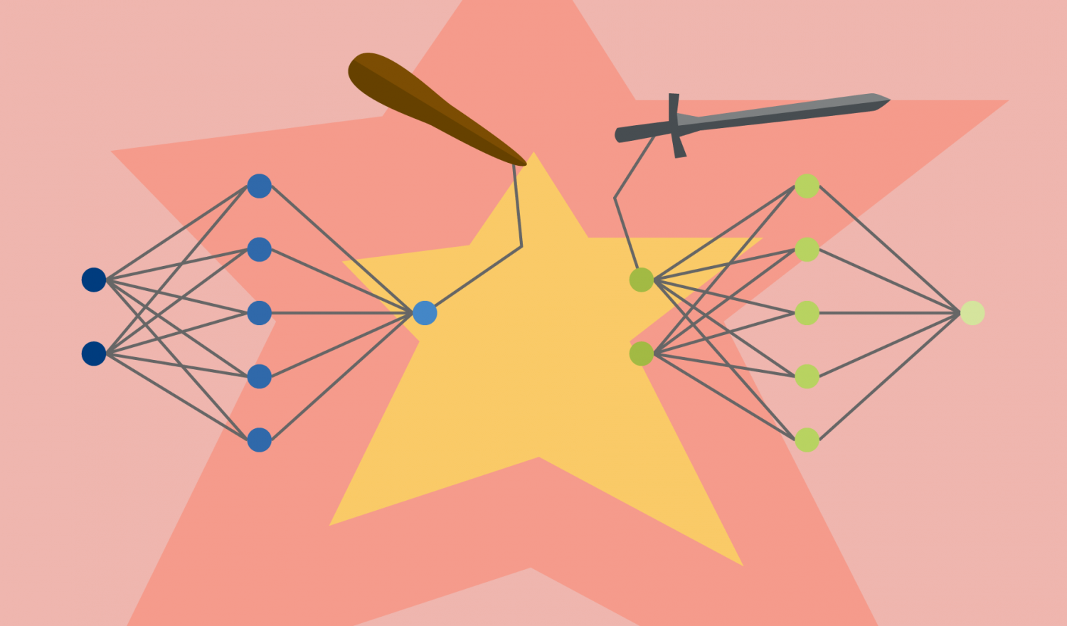
Generative Adversarial Networks were first introduced by Ian Goodfellow et al. on the NIPS 2014 and are a special type of generative model that learns by simulating a game between two players. One player is the so called generator. It tries to generate samples, e.g. images, that resemble the samples of the true underlying distribution of the training set \(p_{data}\). The other player is its adversary, the so called discriminator. It tries to distinguish between the generated fake samples of the generator and the real samples of the training data. So generally speaking the generator tries to fool the discriminator into thinking the generated samples were real while the discriminator tries to determine with high probability which samples are real and which are fake.
Formally we define the generator as
\begin{equation}
x = g(z; \theta_g)
\end{equation}
where \(x\) is the produced sample and \(\theta_g\) are the respective parameters characterizing the generative model. The input to the generator is a noise sample \(z\) which is drawn from a simple prior noise distribution \(p_z\). Often we use a standard Gaussian distribution or a uniform distribution as prior.
The discriminator is defined as
\begin{equation}
d(x, \theta_d)
\end{equation}
where \(\theta_d\) are the respective parameters of the discriminative model and \(x\) is either a real sample \(x \sim p_{data}\) or a fake sample \(x \sim p_g\).
Then the game can simply be expressed as a zero-sum game where the payoff function of the discriminator is given by \(v(\theta_g, \theta_d)\) and the respective payoff for the generator is the exact negative \(-v(\theta_g, \theta_d)\). Accordingly the training is guided by the mini-max objective that can be described as
\begin{equation}
g* = \arg\min_g \max_d v(g,d).
\end{equation}
The natural solution to this game is a Nash equilibrium accomplished by the optimal set of parameters \((\theta_g^*, \theta_d^*)\). Therefore the noise sample \(z\) is transformed by the generator model resulting in a sample \(x \sim p_g\). The ultimate goal of the learning process is to guide the generator by feedback from the discriminator to finally represent the real data distribution in the global optimum.
The Training Procedure
The training objective of a Generative Adversarial Networks is given by the above mini-max equation. For standard GAN the usual choice for the payoff function \(v\) is the cross-entropy:
\begin{equation}
v(\theta_g, \theta_d) = \mathbb{E}_{x \sim p_{data}} \log d(x) + \mathbb{E}_{x \sim p_g} \log (1-d(x)).
\end{equation}
The training consists of a sampling step in which two mini-batches of samples, one with the real values \(x\) and one constituting the generator input \(z\) from the noise prior are drawn. Then the generative transformation is computed and the respective loss is calculated. Next two simultaneous or rather alternating gradient steps are made to minimize the according payoff functions by updating the parameter sets \(\theta_g\) and \(\theta_d\). Any arbitrary SGD based optimization routine can be employed, usually Adam shows good results. At convergence \(p_g = p_{data}\) and the samples of the generator are indistinguishable from the real samples. Consequently the discriminator assigns a probability of 0.5 to all real and fake samples.
Although these theoretical properties are promising, training Generative Adversarial Networks in practice is quite difficult. The difficulty is mostly caused by the non convexity of \(\max_d v(g,d)\) that can prevent the convergence of the GAN which usually leads to underfitting the data. Moreover there is no theoretical guarantee that the game will reach its equilibrium when using simultaneous SGD methods. Thus the stabilization of GAN training remains an open research issue. Careful selection of hyperparameters shows reassuring results w.r.t. to the training and stability of GAN, however the hyperparameter search is often computationally restrictive for complex networks.
Nevertheless GAN show astonishing results, especially in the domain of image generation. A good example is the advanced model developed by the research team of NVIDIA that was trained on the CelebA dataset and transforms statistical noise into fake images of the faces of celebrities:

Realizing that the people on these images do not exist, but were created from noise, one might grasp the enormous potential of GAN based techniques.
Energy-based GAN
Energy-based Generative Adversarial Networks (EBGAN) is a alternative formulation of the GAN architecture. The advantage that is achieved by EBGAN is that much more types of loss functions can be employed compared to the standard GAN that normally only allows to use the binary cross-entropy. To be able to do this the discriminator is interpreted as an energy function. This function maps each point in the input space to a scalar. So basically the discriminator is now used to allocate low energy to regions near the data manifold and high energy to other regions. In this way the energy mass is shaped in the training ultimately forming the surface of the underlying distribution. We can also think of the discriminator as being a parameterized and therefore trainable cost function for the generator. In contrast the generator learns to produce samples that belong to regions which get assigned low energy by the discriminator.
As before the discriminator is served with mini-batches of real and fake samples. Then the discriminator estimates the energy value for each sample by means of a loss function \(\mathcal{L}\). Several loss functions are possible, Zhao et al. use a general margin loss that is given by:
\begin{equation}
\mathcal{L}_d(x,z) = d(x) + \max(0, m-d(g(z))),
\end{equation}
where \(m\) is the margin that is treated as a hyperparameter. Consequently the loss for the generator is:
\begin{equation}
\mathcal{L}_g(z) = d(g(z)).
\end{equation}
The duty of the margin is to separate the most offending incorrect examples from the rest of the data. The most offending incorrect examples are samples that were incorrectly classified and lie very far from the decision boundary, meaning these are the examples with the lowest energy among all incorrect examples. All other examples contribute a loss of 0. In this way the energy surface can be shaped effectively.
Implementations and further reading
With view on the enormous potential and surprising results of Generative Adversarial Networks you can be sure that there are already some projects available on GitHub to dig into the code and to see the real thing in action after digesting the theoretical implications. You can find some nice examples with the links below:
- GAN with TensorFlow tutorial
- Simple implementations of several GAN
- DCGAN
- Comprehensive collection of GAN papers


2 Kommentare