Active Learning in Context of Natural Language Processing – Hands On

In supervised learning it is often all about labels. Do we have enough labeled data? If not, how do we get more? Active learning helps to find the right labels at the right time. It aims to empower a machine learning model to achieve a higher accuracy with less training data. It is a concept that is already well studied in literature and the first papers where published decades ago (http://burrsettles.com/pub/settles.activelearning.pdf). Nevertheless it is becoming more popular in industry nowadays (e.g. prodi.gy). The following blog post is about my findings in active learning that where made working with natural language processing (NLP). I will focus on text classification here.

 

Active Learning

At first, I will shortly go over the theory of active learning and focus only on the pool-based variant here. I can recommend reading http://burrsettles.com/pub/settles.activelearning.pdf if you are interessted in further details. Moreover,  my colleague Matthias wrote a great blog post about active learning that goes into even more theoretical detail..
„The key idea behind active learning is that a machine learning algorithm can achieve greater accuracy with fewer training labels if it is allowed to choose the data from which it learns“ (http://burrsettles.com/pub/settles.activelearning.pdf) Therefore, by using active learning expensive annotations made by a so called oracle, which is normaly a human domain expert, are still needed. But it is possible to reduce training data and still achieve the same or even a higher accuracy.

Pool-Based Active Learning

In the pool-based setting, two separate datasets are used. The first one is the unlabeld pool (U) that can be rather big. Another one is an initialy small labeled set (L) whose size will increase over time. The following illustration shows the pool-based active learning cycle:

 

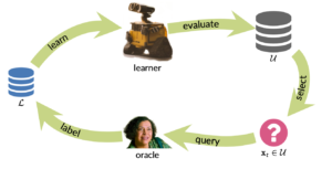
Everything starts by training a machine learning model on L. Afterwards, the trained model makes a prediction for every instance in U. Based on this prediction a query strategy is used to choose which instances should be annotated next. For example, if a machine learning model can produce prediction probabilities (how confident is a model for a single prediction), it is possible to use this information to select the next instance. A simple approach in that case could be uncertainty sampling, that aims to choose the instance in which the model was most uncertain. There exist many more query strategies and approaches to choose the next relevant instances for labeling, e.g. expected error reduction, committee-based algorithms, etc. (https://modal-python.readthedocs.io/en/latest/index.html), which will not be discussed in further detail here. I can recommend reading my colleagues blog post about active learning, if you are interested on more details. But now let’s get a little more practical.

Hands on Active Learning and Text Classification

One major NLP task in many business scenarios is text classification. To resolve this task, it is often all about the data – not the algorithm. (https://blogs.gartner.com/andrew_white/2019/11/12/data-not-algorithm/) Furthermore, gathering good and a high ammount of labeled training data is a cost and time consuming process.

Before we decided as a project team to use active learning for our text classification use cases, we tested and simulated different active learning strategies on a an already full labeled dataset. Our actual model in production that was trained on that dataset has a macro f1-score of 0.95. We wanted to answer the follwing question:
How Many training data could be saved when using active learning?
The instances in our dataset were labeled binary. For illustrative purposes let’s assume that we want to classify sentiments of tweets into good and bad.
We acquired ~40.000 labels for the tweets, which do have a slight label imbalance.
40 % where labeled as bad and 60 % labeled as good.

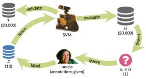
To test active learning, an initial test set of 20.000 tweets was drawn by a random stratified split. The rest forms the unlabeld active learning pool U, that holds also ~20.000 (labeled) tweets. Normally U would not be labeled but due to the fact that we want to simulate active learning, U is also labeled. However, the labels are not used to decide which tweet should be selected for annotation. The next image shows an overview of the simulation process.

Assume we do have our tweets and labels already separeted, we can use scikit’s learn train_test_split method to do the stratified random split:

Initial Training of the Model

To classify the tweets a linear SVM is used with Tf-idf as feature vectors. To speed up the simulation we use the SGD Classifier (https://scikit-learn.org/stable/modules/generated/sklearn.linear_model.SGDClassifier.html#sklearn.linear_model.SGDClassifier) implementation from scikit learn with loss = „hinge“.

The loop is started by training the SGD Classifier with 10 random tweets from the pool set. Both classes appear in this small initial training set to make sure the SGD Classifier can predict both classes. Because we do a simulation, we already have the training labels. Otherwise, it would be necessary to label that data at first. The 10 instances create our inital labeled training set L.

For implementing the whole active learning loop, I can recommend using modAL (https://modal-python.readthedocs.io/en/latest/index.html). It is an active learning framework for python that works well in combination with scikit-learn. ModAL uses a so called ActiveLearner instance which keeps track of L and takes care of querying and teaching new instances.
The following code snippet shows my initialitzation of the ActiveLearner object. It includes an scikit-learn estimator, a query strategy and the features and labels of the initial train set.

The implementation of uncertainty sampling from modal as query strategy is used. Uncertainty sampling ranks all instances in U by the following equation:

?(?)=1−?(?̂ |?)

x represents the instance, ?̂ the prediction of the instance and ?(?̂ |?) the models probability to predict ?̂ for x.
Therefore, the model needs to be able to calculate a probability which is usually implemented in scikit-learn by a predict_proba method of an estimator. The problem is that the SGDClassifier using loss = „hinge“ does not have such a method. To overcome this shortcoming scikit-learn provides the module CalibratedClassifierCV that fits a regressor on a model to interpret the model output as probability.
The follwoing code snippet shows how to use a model wrapper to make SGD Classifier with loss=hinge ready to predict probabilites. The predict_proba function is used in the uncertainty_sampling function provided by modAl.

To simulate and evaluate active learning, another ActiveLearner instance is created that is equal to the active learning instance, except the query strategy is changed to random_sampling.

The ActiveLearner manages the training data and keeps track of the samples put into the training set. By executing the following code, it applies uncertainty sampling on all instances in L (X_pool) and queries the samples where the model is the most uncertain. Calling the teach function adds the given tweets and labels to L and the model is retrained on the newly updated set L. Everything is done in a loop and could be interupted when enough training data is provided.

Results

The following plot provides an answer the question from above:
How Many training data could be saved, when using active learning?

It shows the performance of the SGD Classifiers in every training step. At each time step one annotated tweet is added to the training set. The blue curve represents the scores calculated for the SGD Classifier trained on active learning samples and the red curve shows the scores for the classifier trained on random sampling.

 

 

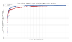
On the y-axis macro f1-score on the test, set is plotted and the number of annotated tweets are shown on the x-axis. Both classifiers are completely refitted on L in each step. Simulation is only done until 10.000 tweets have been annotated because the scores only slowly increase afterwards and training time is increasing in each time step.
Nevertheless, the plot shows that using active learning improves the performance on the test set rapidly. The f1-score saturates faster compared to when using random sampling. After annotating 5.000 tweets, we do have the same performance (f1-score: 0.95) we currently have, using our production model which is trained on far more training data. Even at 10.000 annotated samples random sampling performs not as good as active learning.

Thus, active learning is a complete succes for our tweet annotation task and we aim to implement it in future use cases from the beginning. It helps to reduce the size of the required annotations but keeps the quality of the classifier constant.

Practical Tips

In the last section of this blog post, I will provide some practical tips for using active learning in other use cases.
A good way to start active learning is to run a simulation like I did for our project use case. This is of course only doable if some labeled data exists.
I can recommend trying out different selection techniques besides uncertainty sampling, e.g. query by committee and integrating domain knowledge into the selection process. Density weighting could also help to find more relevant samples.
Furthermore, it is a good practice to draw samples for test and validation sets without active learning because latter evaluation and hyperparameter optimization should be of course done on an unbiased datasets.
Also, in practice, it is often useful to select more than one sample with active learning in an iteration. If human annotators have to wait a long time to annotate because it takes a some time to refit the model and select the next sample, it would not be efficient at all. Thus, I can recommend trying out different query batch sizes, e.g. select the most 100 uncertain samples. In the use case described above, it was found that selecting 100 samples at once performs as good as selecting only one sample per time step.
One more issue to deal with is the fitting of the model in each iteration. Some machine learning models could be continously trained, such as neural networks. This will of course save time because the model has only be trained on the newly labeled data. The problem that arises here, however, is that this could have an impact on the performance of the model. One major problem could be that the model will be overfitted on the new data, which will result in sub optimal results. Therefore, I could recommend to fit the model on all data in L at each timestep. Nevertheless, some techniques do exist to enable continuous learning of machine learning models, especially for neural networks (https://www.researchgate.net/publication/315133141_Fine-Tuning_Deep_Neural_Networks_in_Continuous_Learning_Scenarios, https://arxiv.org/abs/1612.06129, https://openreview.net/pdf?id=ry018WZAZ).

The last point I would like to mention is about the choice of the machine learning model that is used for active learning. Selecting training data with active learning introduces a bias that is created by the model. It is very likely that other models select different datapoints. Thus, a later replacement of the machine learning model could lead to a worse performance compared to a random selection procedure. A good paper that evaluates different model setups for active learning in the context of NLP can be found here: https://www.aclweb.org/anthology/D19-1003.pdf

Over all, giving active learning a chance is still worth it – especially when finding good labeling data points is expensive.