
Federated learning allows a model to be learned from multiple participants without transferring the data to a central location. The approach promises to reduce privacy and latency risks but also has weaknesses such as data quality control and data security.
In this article, we propose integrating a voting protocol with a permissioned blockchain to address several federated learning vulnerabilities. We analyze the performance and robustness of the approach and discuss the results in a predictive maintenance use case. Basic knowledge of federated learning is assumed and can be, for example, looked up in this blog post.
Vulnerabilities in federated learning
Federated learning (FL) has not been as widely integrated into the machine learning community as other ground-breaking technologies because of its vulnerabilities. The vulnerabilities of the FL approach can be divided into security and privacy concerns. Security deals with the correct behavior, integrity, and efficiency of the system against malicious external influences. Furthermore, privacy deals with restricting access and not disclosing data to unauthorized parties. Ideally, each component has access only to the information required to perform its operations. [1,2]
The vulnerabilities of FL can be divided into six domains [1,3]:
- Communication channel: Local and central models are constantly exchanged between clients and the curator. Eavesdroppers can intercept and exchange them for modified models. Another exploitation of this vulnerability is the use of other clients’ models for malicious purposes.
- Gradient leakage: Sensitive information and training data can be revealed through gradient updates during model training.
- Compromised clients can change training parameters and poison the training data or the trained model to perform an attack on the curator.
- A compromised curator can inspect gradient updates from each client and manipulate them, as well as change the central model.
- Aggregation algorithm: In the consequence of compromised participants, a non-robust aggregation algorithm aggregates all models without detecting abnormal updates. This could significantly impact the performance of the central model. Additionally, aggregating a well-performing model which contains a backdoor, would also introduce this backdoor into the central model.
- Finally, the distributed nature of FL allows for collusion between compromised clients, attacks distributed over time, and clients to drop out, meaning clients leave in the middle of a training session.
HyperFlow: Federated learning and blockchain
To address some of the previously mentioned weaknesses of federated learning, Mugunthan et al. [4] propose the integration of the Ethereum smart contract platform, known as BlockFlow. Ethereum is a public blockchain, meaning it is accessible to everyone. This public nature poses a distrust for many use cases. Private blockchains, in turn, are only accessible to select users. In addition, permissioned blockchains are a mix of public and private blockchains that anyone can access, provided they receive permission from the administrators.
In this blog post, we apply the idea of BlockFlow to permission-required blockchains, namely the Hyperledger Fabric blockchain platform, and call this approach HyperFlow.
HyperFlow’s Phases
With the intention of unifying FL and blockchain and thus counteract certain weaknesses of FL, we define HyperFlow in six phases, which are also presented in Figure 1.
- Client Readiness: Clients synchronize their local models with the central model.
- Training: Each client trains a local model with its available data. The model is uploaded to the curator in the cloud, while a corresponding available URL and hash are published to the blockchain.
- Validation: Each client obtains all local models and an availability score is computed for each model. The availability value indicates what proportion of clients were able to successfully obtain the model.
- Evaluation: Models with a high availability score are evaluated by each client using their evaluation data. The evaluation metrics computed are encrypted and published to the blockchain.
- Score decryption: The encryption key used for the computed metrics is provided through the blockchain.
- Aggregation: The evaluated models are aggregated by a weighted average. As weight for the aggregation, the median of the model’s evaluation metrics is used. Models that perform poorly compared to the best-performing model in the current round are removed from the aggregation. This is done by a predefined threshold.

HyperFlow against federated learning vulnerabilities
Although models are encrypted and secure in the cloud, all client models are exposed to all other clients. Furthermore, the models’ aggregation does not avoid the integration of unwanted capabilities to the central model. Hence, we leave the communication channel and aggregation algorithm as not addressed vulnerabilities. In the following, we discuss how HyperFlow addresses four of the six presented vulnerabilities of FL.
Compromised curator
HyperFlow addresses a compromised curator by “decentralizing“ the federated learning approach in a certain way. Each client has access to all models and aggregation scores and can compute its own central model. This is realized by storing local models in the cloud and sharing scores across the Hyperledger Fabric network. The hashes of the models published on the blockchain are used to verify the models. Additionally, the aggregation process of the central model is done by comparing the hashes of the central model across all clients.
Gradient leakage
Differential privacy is a privacy-preserving mechanism for distributed-data processing systems. It preserves the statistical properties of the data while adding statistical noise to them. The privacy achieved can be quantified by the privacy budget spent, which is defined as the bound of how much two adjacent datasets differ. Adjacent datasets can be, for example, data sets that differ by one data point. Since a single data point from the training dataset should never be revealed, a smaller privacy budget can lead to higher privacy. [5]
In an experiment, we use Keras‘ differential private optimizer to achieve privacy-compliant gradient updates. Specifically, we train a long-short term memory (LSTM) model [6-10] that predicts the remaining useful lifetime on NASA’s TurboFan Engine Degradation Simulation data set [11]. Details can be found in the related master thesis.
We evaluated the impact of the privacy budget on the performance of the central model over FL rounds with three, five and ten clients. The privacy budgets used are based on the works of Rahman et al. [12] and K. Wei et al. [13], and the results can be found in Figure 2. A slight increase in the central model’s performance is seen in models trained with an increased privacy budget \(\epsilon\) (lower privacy).

Compromised clients
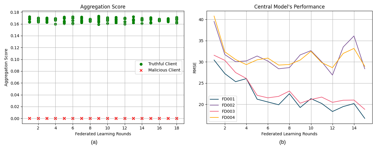
We define compromised clients as participants that share local models which do not increase the central model’s performance. For evaluation purposes, four out of ten clients are classified as malicious and collude with each other. Each malicious client gives a perfect evaluation and validation score to other malicious clients, while truthful clients receive the worst score of zero.
To show a non-robust aggregation of the central model, we have selected a low threshold of 0.3 and present the aggregation scores and the central model’s performance in Figure 3. In Figure 3 (a), truthful clients achieve higher scores than malicious clients. Nonetheless, the scores of malicious clients are not zero, as they perform the same as the baseline when compared to the evaluation records available for truthful clients. Figure 3 (b) shows the performance of the central model in each round of federated learning. After the second round, the impact of malicious clients disrupts the training of the central model.

On the other hand, increasing the threshold to 0.5 sets the aggregation scores of malicious clients to zero. Only models that achieve at least half the score of the best model are considered. Figure 4 (a) shows the aggregation scores of truthful and malicious clients, confirming that malicious clients obtain an aggregation score of zero. The performance of the central model over the subsets of the NASA’s TurboFan Engine Degradation Simulation data set [11] is shown in Figure 4 (b). It shows that selecting well-defined parameters in HyperFlow makes the approach robust against a minority of compromised clients.
Distributed nature of federated learning
The distributed nature of FL opens a door to time-distributed attacks and non-malicious failures. On the one hand, time-distributed attacks are attacks performed on the central model by redirecting the central model into a desired state over FL sessions. On the other hand, non-malicious failures are of heterogeneous nature. For instance, the upload and download of models is prone to network-connectivity failures. In addition, the presence of a bug or interruption in a client’s training pipelines would not be identified by the other clients. Moreover, other failure sources, such as the training resource allocation, machine errors non-related to HyperFlow or power supply, would present challenges for the synchronization of clients over a FL round.
HyperFlow targets non-malicious failures by design, while the aggregation algorithm partly targets time-distributed attacks. Only time-distributed attacks which are measurable by the implemented metrics can be avoided as shown on the analysis of compromised clients. Non-malicious failures reflect as clients dropping-out mid of a FL round. HyperFlow targets these occurrences by setting requirements for the start of a FL session and the synchronization of clients over phases in an FL round. First, a predefined number of participants are required for the beginning of an FL session. Thereafter, each phase of the FL round waits until either a submission deadline is reached or a predefined percentage of clients have submitted their results. Finally, in case none of these conditions is met, the FL session is terminated. The central model is only updated in case the computed session’s model is better-performing than the present central model.
HyperFlows’ blockchain resource consumption
In Hyperledger Fabric there are 4 main components: peer nodes, orderer nodes, the chaincode, and the certificate authority. Each HyperFlow client contains one of each component.
Figure 5 shows the average CPU consumption of each component for a network of three, five, and ten clients. Figure 5 (a) shows exponential increase of workload on peers by the linear increase of clients. This behavior can be seen in the CPU consumption curve of the peers when comparing the increase in consumption in a network with five clients to that of a network with ten clients. The peak of CPU usage for the five clients’ curve is around 60 millicores, while the ten clients’ curve has its peak of around 300 millicores. Figure 5 (b) shows orderers maintain a relatively low CPU consumption since they only package the transactions and forward them to the peer nodes. In the same way, Figure 5 (c) shows the CPU usage of chaincode components is relatively low and rarely surpasses the ten millicores. The certificate authority works to verify components belonging to a specific organization. This is done at the beginning of the blockchain’s application. After that, as shown in Figure 5 (d), the workload of the certificate authority drops to below one millicore.

HyperFlows’ blockchain cost
Using the blockchain’s resource consumption presented, we compare the blockchain costs of HyperFlow to BlockFlow. BlockFlow used a regression model to determine the cost of the Ethereum blockchain for their approach. It is measured in gas, which is defined as one nano Ether. To compute the cost of BlockFlow in relation to the number of clients participating (N) and the federated learning rounds taking place (R), we have
\(Cost_{BlockFlow} = Ether * gas(N, R) * 10^{-9}\),
where we convert gas to Ether, the native Ethereum coin, and multiply it by the current price of Ether in euros.
However, a permissioned blockchain such as Hyperledger Fabric only incurs the cost of running its components. We use the captured resource consumption to calculate the energy consumption of the implementation on a Raspberry Pi [14]. To calculate the blockchain costs of HyperFlow, we integrate the power consumption over time in a federated learning round and multiply it by the number of rounds (R), clients participating (N) and the energy cost in Euros (E), i.e.
\(Cost_{HyperFlow} = E * N * R * \int^{t_{round}}_{0}{P_{Pi}(u) dt}.\)
The subsequent calculations are based on a cost of €2,822.15 per Ether [15] and a cost of €0.2664 per kilowatt-hour [16]. We compare the blockchain costs for a federated learning session of ten clients and ten federated learning rounds for HyperFlow and BlockFlow. BlockFlow has blockchain costs of €1,508.29 while HyperFlow has costs of €7.81. This results in a blockchain cost of approximately 0.52% of the BlockFlow approach for the HyperFlow approach.
Conclusion
In this blog post, we proposed the integration of Hyperledger Fabric, a permissioned blockchain into the Federated Learning process, called HyperFlow. We discussed how HyperFlow can counter some of the weaknesses of federated learning.
First of all, we show that the curator’s responsibilities can be distributed to the clients over a network using the mechanisms of a blockchain. The distributed ledger is used to reach a consensus over the distributed computations and actions available to clients given by a smart contract. Then, we address the gradient leakage vulnerability through the use of differential privacy and show that a slight increase in the central model’s performance is seen in models trained with an increased privacy budget. Third, the collusion of compromised clients to disrupt the central model’s performance is non-effective for a minority of compromised clients as a result of the evaluation round for clients’ models. Last but not least, the vulnerabilities from the distributed nature of FL are reduced by the HyperFlow design and its aggregation algorithm.
In addition, the cost to run HyperFlow is much cheaper than the state-of-the art BlockFlow approach. This is especially because Hyperledger Fabric is a permissioned blockchain. Of course, this also means that the use case must allow this type of Blockchain to effectively take advantage of this benefit. Otherwise, it is unfair to make a comparison between BlockFlow and HyperFlow in terms of their costs.
The blog post was created from a master’s thesis. A detailed elaboration of this topic can be found here.
References
[1] V. Mothukuri, R. M. Parizi, S. Pouriyeh, Y. Huang, A. Dehghantanha, and G. Srivastava. “A survey on security and privacy of federated learning.“ In: Future Generation Computer Systems 115 (Feb. 2021), pp. 619–640. issn: 0167-739X. doi: 10.1016/j.future.2020.10.007.
[2] H. Bae, J. Jang, D. Jung, H. Jang, H. Ha, H. Lee, and S. Yoon. “Security and Privacy Issues in Deep Learning.“ In: arXiv:1807.11655 [cs, stat] (Mar. 2021). arXiv:1807.11655.
[3] N. Bouacida and P. Mohapatra. “Vulnerabilities in Federated Learning.“ In: IEEE Access 9 (2021), pp. 63229–63249. issn: 2169-3536. doi: 10.1109/ACCESS.2021.3075203.
[4] V. Mugunthan, R. Rahman, and L. Kagal. “BlockFlow: An Accountable and Privacy-Preserving Solution for Federated Learning.“ In: arXiv:2007.03856 [cs, stat] (July 2020). arXiv: 2007.03856.
[5] Abadi, M., Chu, A., Goodfellow, I., McMahan, H. B., Mironov, I., Talwar, K., & Zhang, L. (2016, October). Deep learning with differential privacy. In Proceedings of the 2016 ACM SIGSAC conference on computer and communications security (pp. 308-318).
[6] K. T. Chui, B. B. Gupta, and P. Vasant. “A Genetic Algorithm Optimized RNN- LSTM Model for Remaining Useful Life Prediction of Turbofan Engine.“ In: Electronics 10.33 (Jan. 2021), p. 285. doi: 10.3390/electronics10030285.
[7] Y. Wu, M. Yuan, S. Dong, L. Lin, and Y. Liu. “Remaining useful life estimation of engineered systems using vanilla LSTM neural networks.“ In: Neurocomputing 275 (Jan. 2018), pp. 167–179. issn: 0925-2312. doi: 10.1016/j.neucom.2017.05.063.
[8] S. Zheng, K. Ristovski, A. Farahat, and C. Gupta. “Long Short-Term Memory Network for Remaining Useful Life estimation.“ In: 2017 IEEE International Conference on Prognostics and Health Management (ICPHM). June 2017, pp. 88–95. doi: 10.1109/ICPHM.2017.7998311.
[9] A. Listou Ellefsen, E. Bjørlykhaug, V. Æsøy, S. Ushakov, and H. Zhang. “Remaining useful life predictions for turbofan engine degradation using semi-supervised deep architecture.“ In: Reliability Engineering & System Safety 183 (Mar. 2019), pp. 240–251. issn: 0951-8320. doi: 10.1016/j.ress.2018.11.027.
[10] H. V. Düdükçü, M. Taşkıran, and N. Kahraman. “LSTM and WaveNet Implementation for Predictive Maintenance of Turbofan Engines.“ In: 2020 IEEE 20th International Symposium on Computational Intelligence and Informatics (CINTI). Nov. 2020, pp. 000151–000156. doi: 10.1109/CINTI51262.2020.9305820.
[11] A. Saxena and K. Goebel. “Turbofan engine degradation simulation data set.“ In: NASA Ames Prognostics Data Repository (2008), pp. 878–887.
[12] M. A. Rahman, M. S. Hossain, M. S. Islam, N. A. Alrajeh, and G. Muhammad. “Secure and Provenance Enhanced Internet of Health Things Framework: A Blockchain Managed Federated Learning Approach.“ In: IEEE Access 8 (2020), pp. 205071–205087. issn: 2169-3536. doi: 10.1109/ACCESS.2020.3037474.
[13] K. Wei, J. Li, M. Ding, C. Ma, H. H. Yang, F. Farokhi, S. Jin, T. Q. Quek, and H. V. Poor. “Federated learning with differential privacy: Algorithms and performance analysis.“ In: IEEE Transactions on Information Forensics and Security 15 (2020), pp. 3454–3469.
[14] K. Kesrouani, H. Kanso, and A. Noureddine. “A Preliminary Study of the Energy Impact of Software in Raspberry Pi devices.“ In: 2020 IEEE 29th International Conference on Enabling Technologies: Infrastructure for Collaborative Enterprises (WETICE). Sept. 2020, pp. 231–234. doi: 10.1109/WETICE49692.2020.00052.
[15] Coinbase. “Ethereum (ETH/EUR) Preise, Charts und News: Coinbase“. (Apr 2022). url: https://www.coinbase.com/de/price/ethereum (visited on 19/04/2022).
[16] Statista. “Industrial electricity prices including tax Germany 1998-2022“. (Mar 2022). url: https://www.statista.com/statistics/1050448/industrial-electricity-prices-including-tax-germany/ (visited on 19/04/2022).