In order to meet the resource constraints of real-world applications, knowledge distillation is used to compress a larger deep neural network into a more efficient one. Zhang et al. (2018) proposed Deep Mutual Learning (DML), an online distillation algorithm, where multiple networks learn collaboratively. In this article, we compare DML to offline distillation and reveal a consistent instability in the training process.
Motivation
Less than a decade after AlexNet (Krizhevsky et al., 2012) won the ImageNet Large Scale Visual Recognition Challenge (ILSVRC, Russakovsky et al., 2015) in 2012, Deep Neural Networks (DNNs) have become the standard solution for a wide variety of machine learning problems in many different domains. Larger and larger networks continue to push the state of the art, requiring enormous computing and memory capacities. Visual Transformers (Dosovitskiy et al., 2020), for example, are a new, very successful type of network architecture for Computer Vision (CV) that introduces a new order of magnitude in parameter size. However, while the scores achieved with such enormous architectures are impressive, they are far from typical real-life applications, where computational systems only have limited resources. Especially on mobile devices, predictions need to be made fast and with as little computation and memory as possible. This problem is often described as the challenge to deploy (Gou et al., 2021), where we need to bridge the gap between the research and the real-world environment.
For this purpose, a plethora of methods has been introduced in the field of efficient deep learning, optimizing both the inference and the training of DNNs. Here, we focus on distillation algorithms, a type of training pipeline where one network is trained with a transfer of knowledge from another network. Distillation introduces an additional information exchange between multiple networks during the standard supervised learning procedure, which provides more information on the task to the learner(s). Hinton et al. (2015) made it popular for DNNs by the name of Knowledge Distillation (KD), where a high-capacity teacher network is distilled into a lightweight student network. It enables smaller networks, i.e., more shallow with fewer parameters, to perform as well as a high-capacity DNN on the training task. To overcome the requirement of a pre-trained expert model, Deep Mutual Learning (DML, Zhang et al., 2018) uses multiple student networks that learn from each other. Considering this difference, KD is an example for offline distillation, while DML is an online distillation algorithm. All algorithms discussed, as well as our work, focus on the problem of image classification. However, distillation has already proven successful in other problems and domains of deep learning (Gou et al., 2021).
The idea of DML is intriguing: instead of a pre-trained network, all models in the student cohort start without any prior knowledge and learn to solve the task in collaboration. Even more interestingly, the original authors report that the student networks do not only outperform the corresponding architectures trained on the target labels alone but also outperform KD, where a student learns from a static teacher model. They also report that networks trained together as a cohort outperform the same ensemble of networks when each network was trained alone. To summarize their results, the knowledge exchange enables the student cohort to become greater than the sum of its parts, showcasing a significant benefit from online distillation.
With the promising results of Zhang et al. (2018) as a starting point, the goal of this article is to provide an extensive comparison between online and offline distillation. We investigate the theoretical background of DML to see whether it has an elementary advantage over other distillation algorithms. We base our analysis on Menon et al. (2021), which analyses KD from a statistical perspective and gives insight into the mechanics behind it. Furthermore, we complement our theoretical analysis with extensive experiments, comparing DML to KD to understand the differences between online and offline distillation in practice.
Methods
Information Theory
For our comparison of offline and online distillation, we employ concepts of information theory, which we will introduce in the following. The fundamental concept here is entropy, denoted \(H\), of a random variable. It is a measure of uncertainty that quantifies the information, or uncertainty, inherent in the possible outcomes of the variable. It is also called Shannon entropy, in honor of Shannon (1948), and to differentiate it from the concept of entropy in thermodynamics. For a probability distribution on a finite set \(\mathcal{X}\), the Shannon entropy is defined as
\( \begin{align}H(p) & \triangleq\mathbb{E}_p [-\log p] = – \sum_{x \in \mathcal{X}} p(x) \log p(x)\label{eq:entropy}\end{align}\)
where \(x \in \mathcal{X}\) are all possible outcomes of the random variable.
Statistical Distance
In order to compare probability distributions, e.g., outputs of predictive models, we need to establish measures of comparison. Statistical distance quantifies the distance between two random variables or probability distributions.
Let \(p, q\) be probability distributions defined on a finite set \(\mathcal{X}\). We define the following
\(\begin{align}H(p,q) & \triangleq \mathbb{E}_p [-\log q] = – \sum_{x \in \mathcal{X}} p(x) \log q(x)& \hspace{5pt} \text{Cross-Entropy}\\D(p,q) & \triangleq \mathbb{E}_p [\log \frac{p}{q}] = \sum_{x \in \mathcal{X}} p(x) \log \frac{p(x)}{q(x)}& \hspace{5pt} \text{Kullback-Leibler Divergence}\end{align}\)
Both are essential to statistical and specifically to supervised learning, where the loss function \(\ell(h(x), y)\) is a measure of comparison between the output of the model \(h(x)\) and the target \(y\).
Additionally, we see that
\(\begin{align}D(p,q) & = \mathbb{E}_p [\log p] – \mathbb{E}_p [\log q] = – H(p) + H(p,q)\label{eq:equivalence_kld_entropy}\end{align}\)
We use this equivalence for our theoretical analysis. In the following, we write \(p(x)\) as \(p\) for probability distributions, given an input \(x\).
Let us now look at the two distillation algorithms, which we want to compare.
Knowledge Distillation
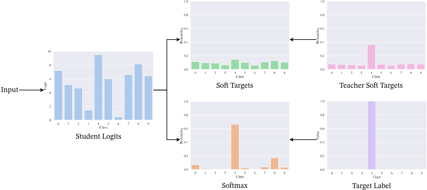
Figure 1: Loss computation for the student network in KD, for one input \(x\). The student outputs a logits distribution over the classes based on the input. For the divergence loss \(D(p_{\tau}^t, p_{\tau}^s)\), temperature smoothing is applied to the logits, which are compared to the soft targets provided by the teacher. For the cross-entropy loss \(H(y,p^s)\), the logits are scaled with Softmax and compared to the target label \(y\).
Hinton et al. (2015) first proposed a simple algorithm for DNNs to transfer the knowledge from a high-capacity teacher network to a small student network, called Knowledge Distillation (KD). To make the student network imitate the teacher’s predictions, the authors add a term to the supervised loss function that is minimized the more similar the output distributions are. They found that it is better to smooth the probability distributions of both networks before comparison. They define soft targets \(p_\tau\) as
\(\begin{align} p_\tau(z_i) = \sigma(\frac{z_i}{\tau}) = \frac{\exp (\frac{z_i}{\tau})} {\sum_j \exp (\frac{z_j}{\tau})}\end{align}\)
where \(z_i\) is the logit for the \(i\)-th class, \(\sigma\) is the Softmax function, and \(\tau \in \mathbb{R}\) is the temperature hyperparameter. We denote the “raw“ output of a neuron in the last layer of the model as logit. \(\tau\) is a hyperparameter that is set before training. Scaling the logits with \(\tau\) is also called temperature smoothing. Using soft targets, they define the distillation loss function for an input-target pair \((x, y)\) as
\(\begin{align}\mathcal{L}_\text{KD} & = (1-\alpha) H(y,p^s) + \alpha D(p_{\tau}^t, p_{\tau}^s)\end{align}\)
where \(p^s, p^t\) are the output distributions of the student and the teacher network, \(H(y,p^s)\) is the cross-entropy between the target labels and the student output, \(D(p_{\tau}^t, p_{\tau}^s)\) is the Kullback-Leibler divergence between the soft targets of teacher and student, and \(\alpha\) is the weighting factor.
The training process is separated into two phases. First, a high-capacity teacher network is trained until convergence in a supervised way on the training dataset. Then, a small student network is trained, optimizing \(\mathcal{L}_\text{KD}\). It performs a unilateral knowledge transfer, as the teacher is trained first, and its weights are fixed during the student training. A schematic visualization of the loss computation can be seen in Figure 1.
This distillation algorithm has later been categorized as offline distillation (Gou et al., 2021) due to the asynchronous learning of the networks. In contrast to it stand online and self-distillation algorithms. In the following, we introduce a prominent example of online distillation, Deep Mutual Learning.
Deep Mutual Learning
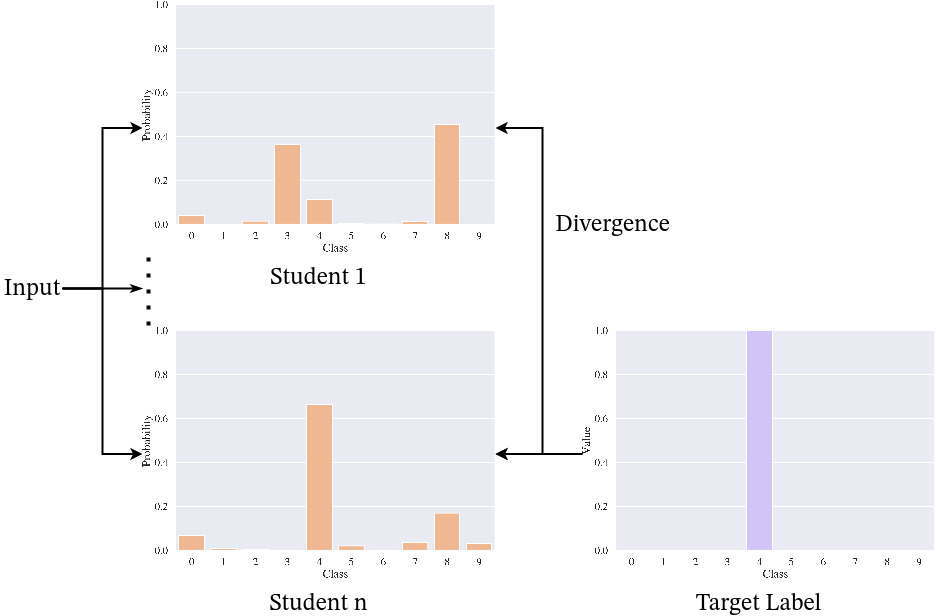
Figure 2: Loss computation for the student network \(n\) in DML, for one input \(x\). Based on the input, each student outputs a probability distribution over the classes. The divergence loss \(D(p^j, p^i)\) is computed comparing the outputs of the other students to output \(n\). The cross-entropy loss \(H(y,p^i)\) is computed with the target label \(y\).
KD can be motivated with an intuition from human learning, where a teacher can help a student to learn a task by providing hints and additional information. The corresponding metaphor for online distillation would then be a study group, where different students have different knowledge backgrounds and help each other learn the task together. Zhang et al. (2018) adapted KD to let student networks learn collaboratively in a one-phase end-to-end training pipeline, termed Deep Mutual Learning (DML). It was the first online distillation algorithm for DNNs (Gou et al., 2021) and has inspired many online distillation methods that followed.
To align the output predictions of the students, DML also uses a two-term loss function, consisting of a supervised loss term and a divergence loss term, also called mimicry loss. Let \(\{p^1, \dots, p^m\}\) be the output predictions of the student cohort of size \(m\) for an input \(x\) with corresponding labels \(y\). Then the DML loss function for the model \(\Theta_i, i \in \{1, \dots, m\}\) is defined as
\(\begin{align}\mathcal{L}_{DML}(\Theta_i) = H(y,p^i) + \frac{1}{m-1} \sum_{j=1, j \neq i}^m D(p^j, p^i)\label{eq:l_dml}\end{align}\)
where \(H(y,p^i)\) is the cross-entropy between the target labels and the output probability distribution, and \(D(p^j, p^i)\) is the Kullback-Leibler divergence between the predictions of \(\Theta_j, j \in \{1, \dots, m\} \setminus \{i\}\) and \(\Theta_i\). Note that \textcite{zhang2018deep} do not use a weighting factor for the two loss terms, nor do they use soft targets for the divergence loss. A schematic visualization of the loss computation can be seen in Figure 2.
As an online distillation algorithm, all networks are trained simultaneously. Each network of the student cohort must start from a different initial condition so that each student learns different features. This is ensured with random initialization for each network. Zhang et al. (2018) provide a visualization of the feature distributions for networks trained separately and with DML, showing that the students indeed learn different features, even when they are trained collaboratively.
Theoretical Comparison
Any deep learning algorithm is only as good as the update steps it takes, so in order to compare KD and DML, investigating the loss function which determines the gradient updates is a good starting point. Reshaping \(\mathcal{L}_{DML}(\Theta_i)\), wee see that
\(\begin{align}\notag \mathcal{L}_{DML}(\Theta_i) &= H(y,p^i) + \frac{1}{m-1} \sum_{j=1, j \neq i}^m D(p^j, p^i) \\\notag &= H(y,p^i) + \frac{1}{m-1} \sum_{j=1, j \neq i}^m \left[ H(p^j, p^i) – H(p^j) \right] \\&= H(y,p^i) + H \left(\bar{p}_i, p^i \right) – \frac{1}{m-1} \sum_{j=1, j \neq i}^m H(p^j). \label{eq:reshaped_l_dml}\end{align}\)
where we define the ensemble prediction \(\bar{p}_i\) for all students except a fixed, but arbitrary \(i \in \{1, \dots, m\}\) as
\(\begin{align}\bar{p}_i = \frac{1}{m-1} \sum_{j=1, j \neq i}^m p^j\end{align}\).
We see that the loss of a student \(i\) is a sum of three terms. First is the cross-entropy between the student prediction and the target label, which remains unchanged by our reshaping. Second is the cross-entropy between the other students‘ prediction (omitting \(i\)) and the prediction of student \(i\), penalizing divergence from the cohort prediction. The last term serves as regularization, where \(– H(p^j)\) is minimized when the cohort predictions are uniform. As we are using gradient descent for the optimization of network parameters, \(\frac{\partial \mathcal{L}_{DML}(\Theta_i)}{\partial \Theta_i}\) is used for a network \(i\) to calculate the update. Here, the last term of the reshaped loss function is omitted, as it does not depend on \(\Theta_i\). To summarize, we see that the third term of the DML loss, the regularization term, has no effect on the optimization of networks with DML.
We now compare DML to KD, as the authors claim that the online distillation algorithm outperforms offline distillation (Zhang et al., 2018). Again, we reshape the loss function for the student network \(\Theta_s\), \(\mathcal{L}_{KD}\) as
\(\begin{align}\notag \mathcal{L}_{KD} (\Theta_s) & = (1-\alpha) H(y,p^s) + \alpha D(p_{\tau}^t, p_{\tau}^s) \\\notag & = (1-\alpha) H(y,p^s) + \alpha \left[ H(p_{\tau}^t, p_{\tau}^s) – H(p_{\tau}^t) \right] \\& = (1-\alpha) H(y,p^s) + \alpha H(p_{\tau}^t, p_{\tau}^s) – \alpha H(p_{\tau}^t). \label{eq:reshaped_l_kd}\end{align}\)
Again, the last term is omitted when calculating the parameter updates with \(\frac{\partial \mathcal{L}_{KD}(\Theta_s)}{\partial \Theta_s}\), as it does not depend on \(\Theta_s\). We see that there are three differences between KD and DML during training. The first difference is the use of weight \(\alpha\) for the two loss terms in \(\mathcal{L}_{KD}\); however, it is usually set to \(\alpha = 0.5\) and is therefore of little interest here. The second two differences lie in the teaching signal, where KD uses soft targets and a pre-trained teacher network to calculate the divergence error. As DNNs tend to be overconfident (C. Guo et al., 2017), it is a good rule of thumb to add temperature smoothing when using KD, which is why it is so successful. The fact that DML does not use soft targets is not a disadvantage in itself, as randomly initialized networks in the process of training provide the teaching signal here. However, it requires an empirical analysis to see whether the cohort is a good teacher.
Empirical Comparison
For our empirical comparison, we implement the two algorithms according to the original papers and compare them on a standard image classification dataset, Fashion-MNIST (Xiao et al., 2017). Let us first present our experimental setup and continue with the results.
Experimental Setup
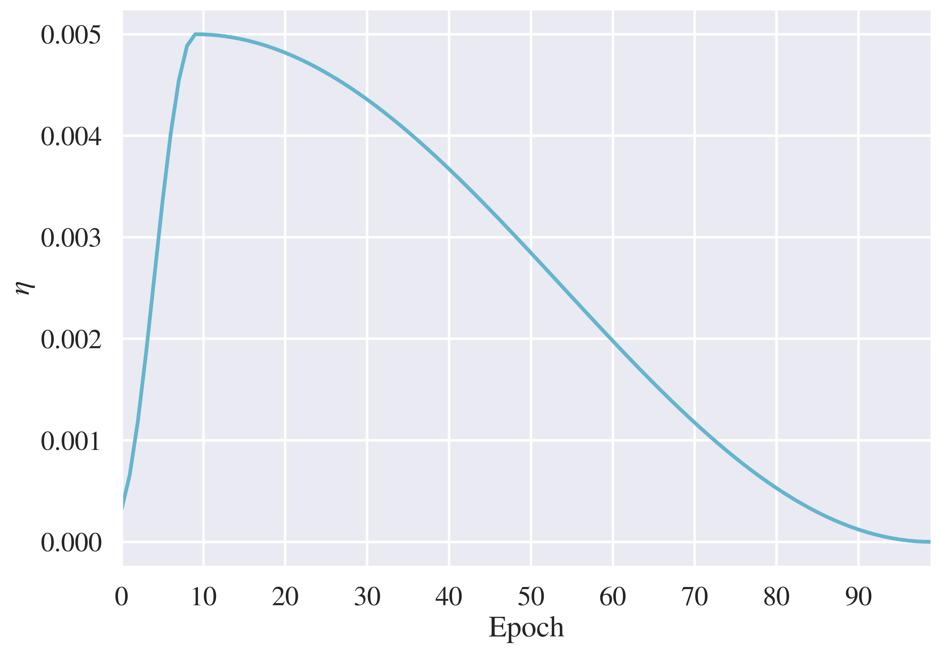
Figure 3: Cyclical learning rate schedule over the course of training, with a maximum learning rate \(\eta = 0.005\) after 10% of the total epochs.
The dataset used is Fashion-MNIST (Xiao et al., 2017), an image classification dataset consisting of \(28 \times 28\) greyscale images of 70 000 fashion products from 10 categories, with 7 000 images per category. The dataset is structured identically to the popular MNIST dataset (LeCun et al., 1998) but poses a more challenging classification task. It is split into 60 000 images for training and 10 000 images for testing, with an equal distribution of the classes in both sets.
All the networks used in the experiments are Residual Networks (ResNets, K. He et al., 2016), a popular class of CNN architectures for image data. We use two architectures, namely ResNet-18 and ResNet-50, the number referring to the number of layers of the network. Both have been proposed by the original authors. The more lightweight ResNet-18 consists of 2-layer residual blocks and is used as student architecture, while ResNet-50 uses 3-layer blocks and serves as architecture for the teacher in KD.
We train five runs with 100 epochs for each hyperparameter configuration, with a batch size of 1024. The networks are initialized identically at the beginning of each run. We test two hyperparameter configurations:
- Adam optimizer (Kingma & Ba, 2014) with a learning rate of \(\eta = 0.01\)
- AdamW optimizer (Loshchilov & Hutter, 2017) with a cyclical η with maximum η = 0.005, adapted from the super-convergence learning rate schedule (Figure 3, Smith and Topin, 2018).
A learning rate schedule with a warm-up phase at the beginning of training, i.e., starting with a lower learning rate and gradually increasing it, prevents early overfitting to spurious patterns due to the random choice of the first mini-batches (Goyal et al., 2017).
Results


Figure 4a and 4b: Validation accuracy over 100 epochs for both hyperparameter settings on Fashion-MNIST. Each line shows the mean for the respective algorithm over five runs, while the shading shows the standard deviation.
In the first hyperparameter setting, the baseline and KD surpass 89 % accuracy. The best models are both KD variants, with a ResNet-18 and a ResNet-50 teacher, which achieve 89.5 % accuracy. DML does not achieve stable results, as not only the average accuracy is much lower for the cohort, but the confidence interval is also an order of magnitude larger than for the other algorithms. Figure 4.a illustrates the instability of DML. The high variance is caused by student networks “crashing“, i.e., dropping to guessing accuracy at some point during training and not improving anymore. However, even when that happens, the other networks are still optimized to minimize the divergence from the failing model. As a result, the divergence loss becomes contrary to the cross-entropy error calculated with the target labels. It can be regarded as noise in the loss signal. As a result, the best student in the cohort does not reach as good results as the other models, scoring 82.6 % accuracy on average.
In the second hyperparameter setting, we address the shortcomings of the algorithms we found in the first experiments. This includes a more refined learning rate schedule with a lower learning rate and a different optimizer for all algorithms. Illustrated in Figure 4.b, DML now achieves an accuracy comparable to the other algorithms. The average accuracy of all algorithms now lies between 87 % and 89 %. The cyclical learning rate schedule, together with a lower learning rate, stabilizes DML enough so that students do not “crash“ anymore. Therefore, the divergence loss is minimized together with the target loss, and helps the students to achieve a higher accuracy.
Discussion
Evaluating the performance of the different distillation algorithms on Fashion-MNIST, we better understand the mechanics of the distillation schemes and build on the theoretical analysis. Most importantly, DML did not perform as well as expected, based on the promising results reported by Zhang et al. (2018). More specifically, the learners suffer from instability in training, where one or more student networks in a cohort “crash“, i.e., the predictions fall back to guessing at some point during training and do not improve anymore. While using a cyclical learning rate schedule, a lower learning rate, and a different optimizer remedy the instability, the distillation from peers introduces a source of uncertainty that impairs the cohort’s performance. KD on the other hand, demonstrates the positive effect that can be gained from distillation, as it successfully outperforms the baseline in both hyperparameter configurations. It should be noted that we also experimented with various extensions to DML, none of which achieved the baseline performance.
Greater than the sum of its parts?
The idea of knowledge emerging in the student cohort from collaborative learning, as suggested in the results of Zhang et al. (2018), motivated us to research the mechanics of online distillation. Our conclusion from this work is that DML does not add an improvement over the baseline trained on the target labels, nor over KD. Instead, DML introduces instability into the training process, which impairs the convergence of the students in the cohort.
The idea of peer networks learning from each other, rather than from a teacher network, still seems intriguing. However, to the best of our knowledge, we have tried all straightforward modifications of the algorithm to stabilize the training. One direction to explore would be to exclude poorly performing students from contributing to the distillation loss, similarly to Q. Guo et al. (2020).
References
Dosovitskiy, A., Beyer, L., Kolesnikov, A., Weissenborn, D., Zhai, X., Unterthiner, T., … & Houlsby, N. (2020). An image is worth 16×16 words: Transformers for image recognition at scale. arXiv preprint arXiv:2010.11929.
Gou, J., Yu, B., Maybank, S. J., & Tao, D. (2021). Knowledge distillation: A survey. International Journal of Computer Vision, 129(6), 1789-1819.
Goyal, P., Dollár, P., Girshick, R., Noordhuis, P., Wesolowski, L., Kyrola, A., … & He, K. (2017). Accurate, large minibatch sgd: Training imagenet in 1 hour. arXiv preprint arXiv:1706.02677.
Guo, C., Pleiss, G., Sun, Y., & Weinberger, K. Q. (2017, July). On calibration of modern neural networks. In International Conference on Machine Learning (pp. 1321-1330). PMLR.
Guo, Q., Wang, X., Wu, Y., Yu, Z., Liang, D., Hu, X., & Luo, P. (2020). Online knowledge distillation via collaborative learning. In Proceedings of the IEEE/CVF Conference on Computer Vision and Pattern Recognition (pp. 11020-11029).
He, K., Zhang, X., Ren, S., & Sun, J. (2016). Deep residual learning for image recognition. In Proceedings of the IEEE conference on computer vision and pattern recognition (pp. 770-778).
Hinton, G., Vinyals, O., & Dean, J. (2015). Distilling the knowledge in a neural network. arXiv preprint arXiv:1503.02531, 2(7).
Krizhevsky, A., Sutskever, I., & Hinton, G. E. (2012). Imagenet classification with deep convolutional neural networks. Advances in neural information processing systems, 25.
LeCun, Y., Bottou, L., Bengio, Y., & Haffner, P. (1998). Gradient-based learning applied to document recognition. Proceedings of the IEEE, 86(11), 2278-2324.
Menon, A. K., Rawat, A. S., Reddi, S., Kim, S., & Kumar, S. (2021, July). A statistical perspective on distillation. In International Conference on Machine Learning (pp. 7632-7642). PMLR.
Russakovsky, O., Deng, J., Su, H., Krause, J., Satheesh, S., Ma, S., … & Fei-Fei, L. (2015). Imagenet large scale visual recognition challenge. International journal of computer vision, 115(3), 211-252.
Smith, L. N., & Topin, N. (2019, May). Super-convergence: Very fast training of neural networks using large learning rates. In Artificial intelligence and machine learning for multi-domain operations applications (Vol. 11006, p. 1100612). International Society for Optics and Photonics.
Xiao, H., Rasul, K., & Vollgraf, R. (2017). Fashion-MNIST: a novel image dataset for benchmarking machine learning algorithms. arXiv preprint arXiv:1708.07747.
Zhang, Y., Xiang, T., Hospedales, T. M., & Lu, H. (2018). Deep mutual learning. In Proceedings of the IEEE conference on computer vision and pattern recognition (pp. 4320-4328).