Deep neural networks are generally considered black boxes: We often do not understand which input features a model’s decisions are based on. Explainable Artificial Intelligence (XAI) techniques promise to offer a peek inside the box – but how robust are they? In this blog post, I am going to show you how to hide an adversarial attack on images by manipulating their explanations to make them appear “unsuspicious.“
Motivation
Nowadays, deep learning models are used in many different areas, even safety-critical ones such as autonomous driving. However, these systems do make mistakes from time to time, which can have grave consequences: Since 2018, Teslas running on “Autopilot“ have crashed into parked emergency vehicles about a dozen times in the United States, thereby injuring multiple and even killing one passenger. The National Highway Traffic Safety Administration (NHTSA) has since picked up an investigation into the accidents.
When I read about this, I asked myself whether it was possible for a data scientist at Tesla to somehow hide the shortcomings of their model, so that the auditors would come up empty-handed. I imagined the following – hypothetical – scenario: The data scientist investigates the model failure and finds out that emergency vehicles are consistently misclassified as pedestrian crossings by the computer vision system, causing the cars not to behave as expected. They decide to manipulate the images captured right before the crash with the goal of having them classified as emergency vehicles by the model, thus effectively hiding the error. However, they also know that the auditors will use particular XAI techniques in their investigation and are worried that the manipulation will be uncovered due to suspicious explanations created based on the attacked images. As a result, they decide to also manipulate the model in order to create explanations for the attacked images that look very similar to the ones of the original images, while at the same time making sure both original and attacked images are still classified as their corresponding target class label. This way, the manipulation can effectively be hidden “in plain sight“.
Basics
Based on the hypothetical scenario described above, I came up with a multi-step approach to manipulate both input images and model. In the next sections, I will briefly describe the initial steps taken before diving into the central aspect: the adversarial fine-tuning.
Dataset & model
For my experiments, I decided to use the Fashion-MNIST dataset and a rather simple Convolutional Neural Network (CNN) classifier. The Fashion-MNIST data set was created by Zalando and contains 70000 fashion items in 10 different categories, e.g. sandal, trousers, dress, etc.. The images are rather small (32×32 pixels) and come in 8-bit grayscale format.
The CNN classifier I used is based on an example architecture provided in the PyTorch GitHub repository which I simply reimplemented using PyTorch Lightning. It consists of two convolutional layers with 3×3 kernels, followed by two fully connected layers. The model contains ReLU activations in all but the last layer which instead uses the Softmax. It also includes a max-pooling layer after the convolutional layers and two Dropout layers. The image below shows an overview of the architecture.

I trained the model on the Fashion-MNIST training set for 25 epochs with a batch size of 64 using the Adadelta optimizer. The initial learning rate was set to 1.5 and statically decreased every epoch by a factor of 0.85. After training, the model achieved an accuracy of 93.03 % on the standard Fashion-MNIST test set.
Adversarial attack on the data
Unfortunately, CNN models are easily fooled: By changing a few pixels in an input image, the model can be tricked into classifying the image as a completely different category. There are various ways to adversarially attack images based on an image classifier. In my thesis, I used the so-called DeepFool technique [Moosavi-Dezfooli et al., 2016], which is an iterative attack technique based on linearizations of the model’s decision hyperplanes.
In my experiment setup, I attacked all images of the Fashion-MNIST data set based on the CNN classifier trained earlier. All successfully attacked images (from now on called adversarials) were then saved as PyTorch tensors together with their adversarial labels. The images, for which the attack did not work, were not used in the next steps.
Creating the visual explanations
As initially described, Explainable Artificial Intelligence (XAI) techniques are used with the goal of making the predictions of a model and how they relate to the input features more understandable. The field of XAI offers a rich taxonomy and many different ways for creating these explanations. In my thesis, I concentrated on visual XAI methods that are based on the gradient of the model’s output with respect to a particular input image or intermediate feature representations. The techniques I chose are called Gradient-weighted Class Activation Mapping (Grad-CAM) [Selvaraju et al., 2017] and Guided Backpropagation [Springenberg et al., 2015]. You can refer to this article to learn more about them.
I created visual explanations for all the original and adversarial Fashion-MNIST image pairs and their corresponding labels. For this, I used the Python library Captum which offers implementations of various XAI techniques for PyTorch models. In Figure 2, you can see an example of the original and adversarial explanations created using Grad-CAM and Guided Backpropagation.
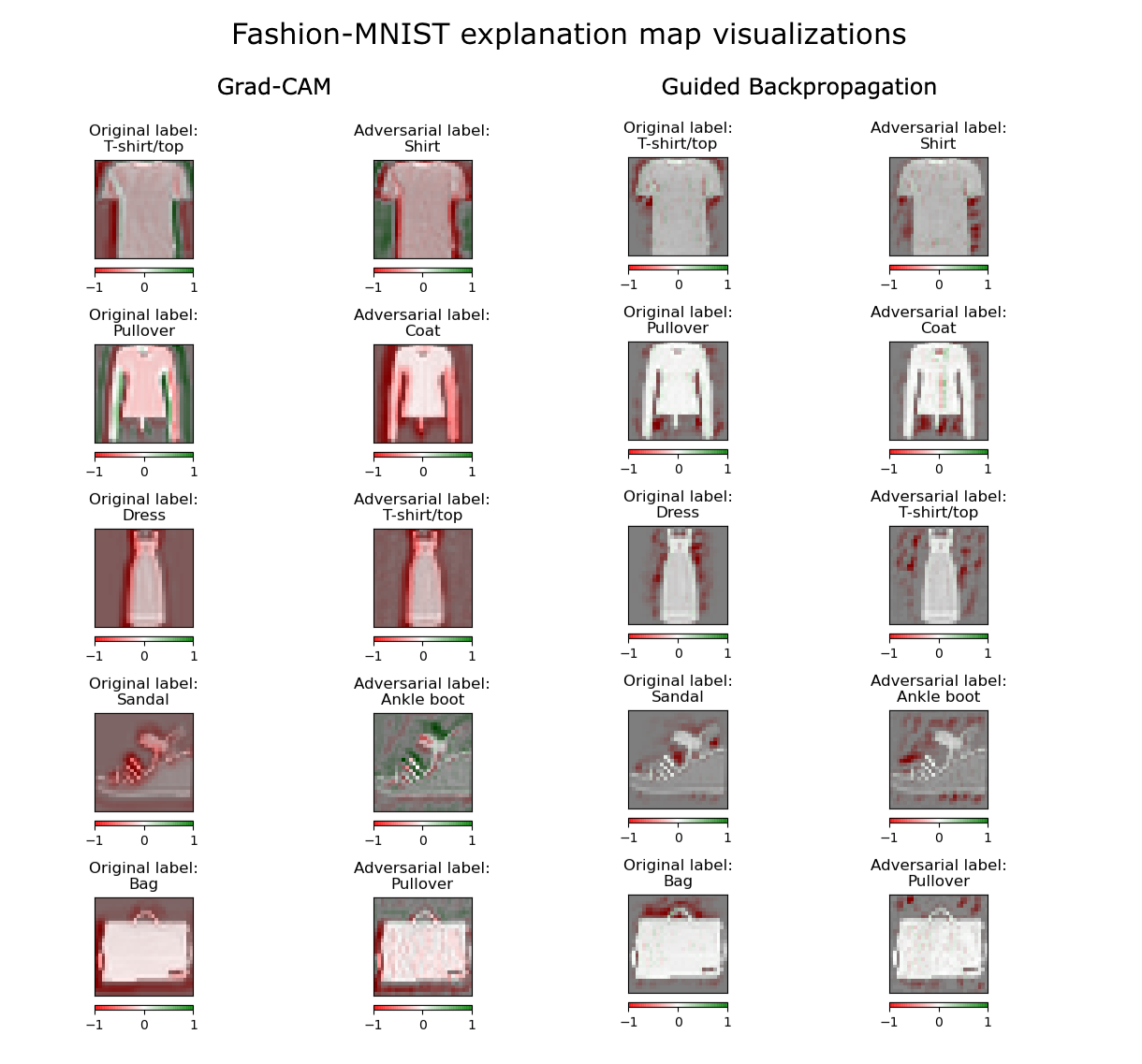
Noticeably, some of the originals (first and third columns) and adversarials (second and fourth columns) look very distinct – and this is what I wanted to change with my adversarial fine-tuning procedure: One of the goals of my thesis was to make the adversarial explanations look “unsuspicious“, meaning that they should be visually similar to the original explanations, even though they were created based on a different class label. In the next section, you’ll find out how this can be achieved.
Adversarial fine-tuning
The adversarial fine-tuning represents the central part of my thesis and is based on the results of the previous steps, namely the CNN model, the original and adversarial images (+ labels), and the corresponding visual explanations. As you may recall, in the hypothetical scenario described at the start, the malicious actor wants to hide the adversarial attack on the images from the auditors. I have attempted to do the same by setting the following goals for the manipulation:
The manipulated model needs to…
- retain the classification performance on the original Fashion-MNIST images,
- consistently (mis-)classify the adversarial images as their initial adversarial class label, and
- produce explanations for original and adversarial image pairs that are visually similar.
In the next section, I will introduce the composite loss function I came up with to formalize these requirements.
Composite loss function
The cross-entropy loss is a popular choice for single-target classification tasks. It is used with models that output a probability score between 0 and 1 for each class. A low cross-entropy value indicates that the predicted class probability is close to the true class probability (which is what we want). On the other hand, the cross-entropy value of a class will be high if it was assigned a high probability even though it is not the ground truth class, or if the predicted probability of the ground truth class is low.
As in goals 1 and 2 mentioned, before retaining the classification performance of the model on original and adversarial images, the cross-entropy loss can be used in both cases. The first loss term \(L_{CE_{Orig}}\) takes into account all original images and their ground truth labels to make sure that the model still works correctly on the unaltered data instances after the manipulation. The second loss term \(L_{CE_{Adv}}\) is used on a subset of the adversarial images, namely the ones whose original counterpart belongs to a certain target class \(y_t\). The reason why I chose to include only a part of the adversarials is that I believe it is more likely that a malicious actor would want to manipulate the model with respect to a particular image class rather than all of them.
The third goal specifies that the explanations of original and adversarial image pairs should be visually similar. Again, similarly to the second loss term, this term is applied only to a subset of the data, namely the pairs of explanations of original and adversarial images whose original labels belong to target class \(y_t\). As my model manipulation targets only one class, it makes sense to only try and obscure the attack on data instances related to this particular class.
In order to quantify and improve the “visual similarity“ between two explanations, I tried out two different loss metrics: the Mean Squared Error (MSE) and the Pearson Correlation Coefficient (PCC). The MSE can simply be minimized together with the two cross-entropy loss terms, as smaller values indicate less difference and thus a higher similarity between the pixels of the two explanation images. The PCC, however, represents a measure of linear correlation in the range of [-1, 1], where -1 indicates perfect negative and 1 perfect positive linear correlation. In order to use this metric as a basis for the loss term, I decided to limit its range to only positive values and subtract the result from one to be able to minimize it during training:
\(SIM_{PCC}(h_1, h_2) = 1 – max(0, PCC(h_1, h_2))\)
My initial experiments showed that the similarity loss based on the PCC metric works well for my task, as minimizing the term above also yields visually similar-looking explanations. The MSE, on the other hand, did not yield very good results: After a few training epochs, the explanations already diverged from one another and visual artifacts started appearing. You can see an example of this in Figure 3, where the adversarials, in particular, seem to undergo undesired changes:

Based on these initial results, I decided to go with the PCC-based loss. Without using too much mathematical notation, my final similarity loss term \(L_{SIM}\) looks like this:
\(L_{SIM} = \frac{1}{2} \left( SIM_{PCC}(h_{orig}, h_{adv}^{*}) + SIM_{PCC}(h_{orig}, h_{orig}^{*}) \right) \)
The first term inside the brackets calculates the PCC-based similarity between the original explanation before the manipulation (\(h_{orig}\)) and the adversarial explanation after the manipulation (\(h_{adv}^{*}\)). It ensures that the adversarial explanation will look similar to the initial original explanation and hence “unsuspicious“. The second term represents the similarity between the pre- (\(h_{orig}\)) and post-manipulation (\(h_{orig}^{*}\)) original explanations. I added this term in order to prevent the original explanations from changing too much due to the model manipulation. The similarity loss term can now be minimized together with the other components.
The whole composite loss function has the following form:
\(L = L_{CE_{Orig}} + L_{CE_{Adv}} + \gamma L_{SIM}\)
The \(\gamma\) parameter is a weighting factor that can be used to change the influence of the similarity loss term on the training. In my experiments, I found that setting \(\gamma=1.0\) and hence giving it the same influence as the cross-entropy terms usually led to good results.
Choosing target classes for the manipulation
As mentioned earlier, I based the approach on a target class \(y_t\), meaning that only the adversarial counterparts of originals belonging to that target class were subjected to the manipulation.

This left me with the task of deciding which classes I wanted to base the manipulation on. I figured that it would make sense to choose the ones that would be the “easiest“ and “hardest“ to manipulate and formalized this requirement by picking the classes with the highest and lowest initial PCC-based similarities regarding their original and adversarial explanations. The box plots in Figure 4 show these explanation similarities for all Fashion-MNIST classes for both Grad-CAM and Guided Backpropagation:
As you can see, Sandal and Coat are the top and bottom classes for Grad-CAM, while the exact opposite is true for Guided Backpropagation. I figured the top class would be easiest, and the bottom class the hardest to manipulate.
Replacing ReLU with Softplus activations
Rectified Linear Units are a very popular activation function choice in deep learning architectures due to their piece-wise linearity. However, this also comes with a downside: They do not have a second derivative [Dombrowski et al., 2019]. This is a problem in my case, as the XAI techniques use the gradient (first derivative) to create explanations. In order to know in which direction the model weights need to be changed to produce explanations that are more similar, the second derivative is needed as well.
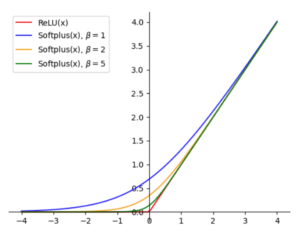
The solution proposed by Dombrowski et al. includes replacing the ReLU activations with Softplus activations of the form:
\(Softplus(x) = \frac{1}{\beta} log(1+e^{\beta x})\).
For larger values of \(\beta\), the Softplus closely approximates the ReLU function but has a well-defined second derivative. The plot in Figure 5 shows the ReLU function and Softplus functions using different values of \(\beta\).
For my adversarial fine-tuning, I set \(\beta=30\) because the corresponding model achieved the same classification performance as the one using ReLUs. During the test stage, I reintroduced the original ReLU activations.
Evaluation metrics
After running the fine-tuning, I needed to assess whether the three goals I defined earlier were met. For this, I used the following metrics:
- Accuracy / adversarial misclassification rate: Accuracy is a standard metric to assess the classification performance of a model. The adversarial misclassification rate is in essence a custom accuracy metric, but one used specifically for assessing how many of the adversarials were (successfully) misclassified by the model. I use this metric to assess the performance on the adversarials whose original counterparts belong to the target category \(y_t\).
- PCC, MSE, and Structural Similarity Index Measure (SSIM): These three metrics are also used in related works (e.g. [Dombrowski et al., 2019]) to assess the similarity between visual explanations. For PCC and SSIM higher values indicate higher similarity, while for the MSE it is the opposite. Using these metrics, I compare the similarities between the original and adversarial explanations before and after the manipulation to see whether they have been increased.
Results
Classification performance
As specified by goals 1 and 2, the accuracy and adversarial misclassification rate should not deteriorate after the manipulation. The table in Figure 6 displays the classification performance of the model before (columns pre) and after (columns post) the manipulation on each combination of XAI technique and target class. Mind that the post-manipulation results are calculated based on k-fold cross-validation runs with k=5 and hence always include the mean and standard deviation:
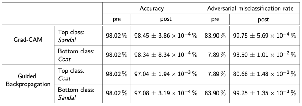
As can be seen, the accuracy actually improved slightly for both the manipulations based on class Sandal and Coat when manipulating the Grad-CAM explanations. For Guided Backpropagation, however, the accuracy deteriorated by close to 1 % in both cases. The adversarial misclassification rate was improved by a large margin in all of the manipulations.
It seems that it is generally possible to achieve goals 1 and 2, with the small addition that there could be a slight deterioration in accuracy on the original data. But who knows, maybe someone can improve this in the future?
Explanation similarities
Grad-CAM

So how did my approach fare regarding goal 3. of increasing the similarity between original and adversarial explanations?
In Figure 7, you can see the results for all similarity metrics before and after the manipulation based on Grad-CAM and both Sandal and Coat.
The box plots show that the explanation similarity increased for both classes after the manipulation across all metrics (mind, however, that the mean SSIM (orange triangle) decreased for Sandal while the median increased). For the PCC metric of class Coat this change is especially large: the median (black line) changed from -0.97 to 0.88 and the mean from -0.87 to 0.34. Visibly, the post-manipulation PCC values show a large spread, indicating that there are still many explanations that display a low similarity.
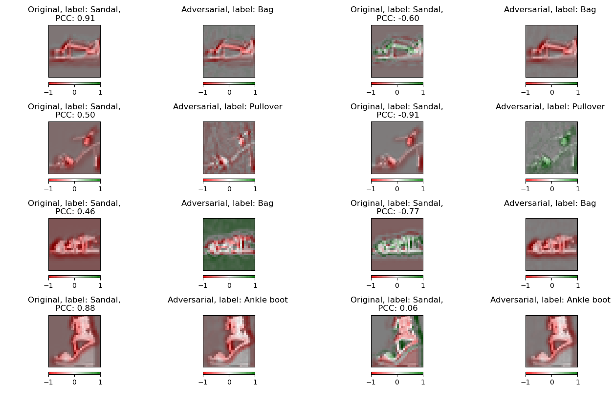
Now let’s look at some qualitative results. Figure 8 displays the largest positive change in PCC explanation similarity based on Grad-CAM for class Sandal.

Visibly, the original and adversarial explanations look very distinct before the manipulation which is also indicated by the strong negative linear correlation according to the PCC metrics displayed above the originals. After the manipulation, the explanations have changed in a way to make them look almost identical, also indicated by the high PCC values.
To get a full picture, we also need to look at the opposite cases, meaning the explanations that changed for the worse. In Figure 9, you can see the largest negative changes in PCC explanation similarity. Here, it becomes apparent that the manipulation did not work as expected for all samples. As you can see in the first row, the initial explanations of original and adversarial were quite similar. However, the manipulation led to a profound change in the original explanation, hence decreasing the similarity.
Guided Backpropagation
For Guided Backpropagation, the situation was a bit different, as the manipulation seemed to work well for class Sandal, but not for class Coat, which is shown in Figure 10.
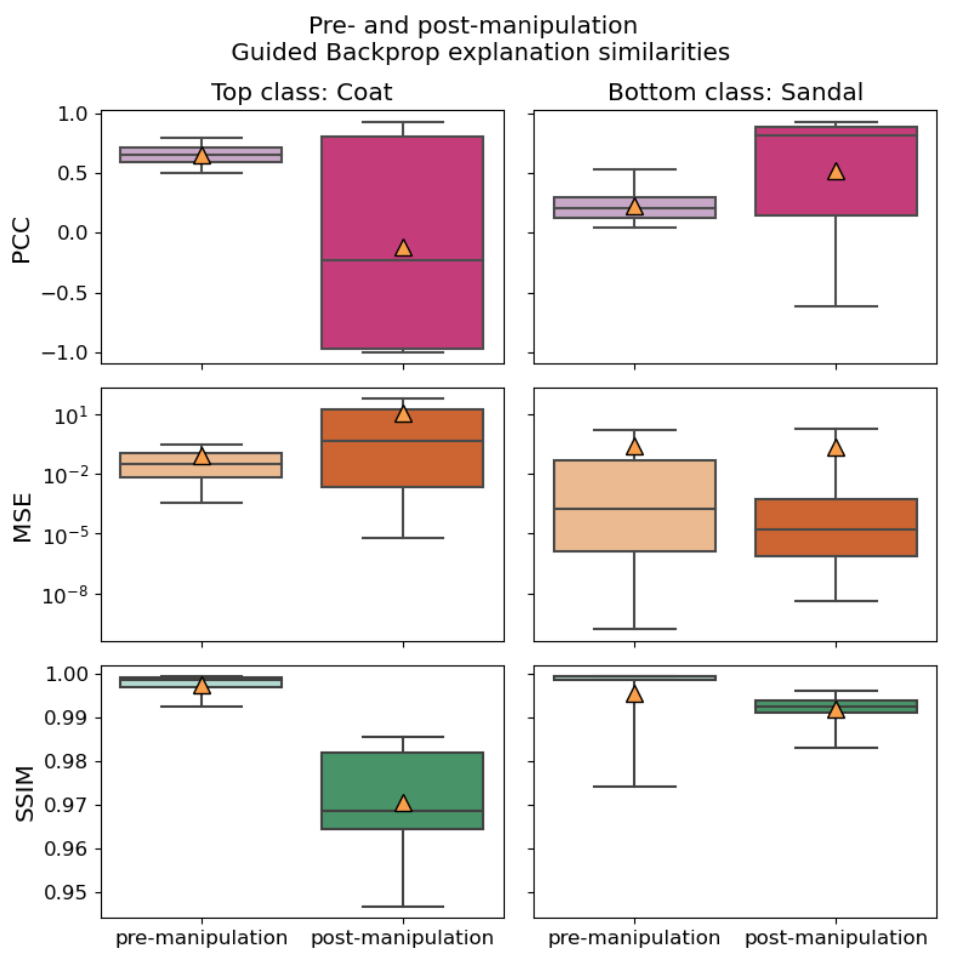
On the right-hand side, you can see that both the PCC and MSE similarities saw some improvement for class Sandal. For class Coat, on the other hand, there was a significant deterioration: The explanations of original and adversarial images are less similar after the manipulation than before across all three metrics. I investigated this issue in an ablation study by using the weighted cross-entropy loss (see parameter weight in the PyTorch docs) as the first loss term and assigning different weights to class Coat while leaving the weights of the other classes at 1. This means that I put more emphasis on the model to get this class right. Upon inspecting the results, I noticed that the higher I chose the weight, the better the classification performance of the manipulated model became. However, there was an inverse relationship with the explanation similarity, leading it to become lower as I chose higher weights. Apparently, for this particular Fashion-MNIST class, I cannot have my cake and eat it too. 😉
Additional results
Because I had some time left towards the end of my thesis, I also wanted to know whether I could achieve good results for other Fashion-MNIST classes with the two XAI methods I chose and whether it is possible to manipulate other XAI methods in the same way.
Regarding the first case, I tried to manipulate the classes Trousers, Dress, as well as both of them combined. Without much hyperparameter tuning (rather, I just guessed which parameters could work well) I got quite decent results as you can see in Figure 11 for Grad-CAM.

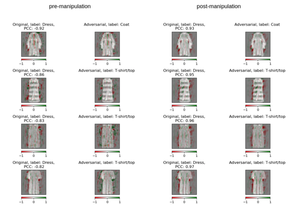
Astonishingly, the manipulation also worked for the XAI techniques Gradients * Inputs and Integrated Gradients. In the following picture, you can see some example manipulation results for Integrated Gradients on target class Dress. After the manipulation, the explanations look astonishingly similar (see Figure 12).
Summary & conclusion
To summarize, I can say that most of the adversarial fine-tuning experiments I conducted in my thesis were quite successful. The three main goals of 1) retaining the classification performance on the original images, 2) ensuring the adversarial images are consistently misclassified, and 3) manipulating the model in such a way that the original and adversarial explanations look very similar, could be achieved in most of the cases. Only while manipulating based on Guided Backpropagation and class Coat was I not able to adhere to all of the goals.
Generally, these findings are in line with previous works by Dombrowski et al., Ghorbani et al. and Heo et al., who also manipulated explanations, but took approaches that differ from mine. You should definitely check their works out though if you want to know where I got the inspiration from!
Finally, all of these results in the space of attacking XAI techniques leave us with a few open questions:
- Which other XAI techniques can be manipulated in this way?
- Can we come up with a standardized and reproducible approach to evaluate the robustness of XAI techniques?
- And what are the implications of these findings for the use of XAI techniques outside of scientific research?
I hope this post was able to spark your interest in attacks on Explainable Artificial Intelligence – I for my part am excited to see what directions the research in this area takes and how this in turn will affect machine learning applications in the future.
References
GitHub repository
- You can find the code for the master thesis in the following GitHub repo: https://github.com/inovex/hiding-adversarial-attacks
Papers
- [Moosavi-Dezfooli et al., 2016] – DeepFool: A Simple and Accurate Method to Fool Deep Neural Networks
- [Dombrowski et al., 2019] – Explanations can be manipulated and geometry is to blame
- [Selvaraju et al., 2017] – Grad-CAM: Visual Explanations from Deep Networks via Gradient-based Localization
- [Springenberg et al., 2015] – Striving for Simplicity: The All Convolutional Net
