All supervised machine learning is based on three components: Data, labels and a learning algorithm that learns a model from the data and the labels. Both data and learning algorithms are usually not an issue; data is abundant and there is an ever-growing body of well understood learning algorithms to choose from. The real impediment to successful machine learning projects are the labels, or rather the lack thereof.
Academic research often focuses on huge labeled datasets like ImageNet or the OPIEC corpus, but when you are building customer specific solutions, e.g., for fraud detection or price prediction, you can count yourself lucky if you are given even a handful of labels. More often than not, additional data has to be labeled in a time-consuming and thus costly process. Worse, because labeling is tedious and tiring, it is a error-prone and may lead to sub-optimal prediction models. Whats more, many of the labels may not actually useful for the learning algorithm, because other labels already exist for similar data or the data is in regions far away from the decision boundaries. Is there a better way to do this? As it turns out, there is: Active Learning.
In Active Learning, the learning algorithm is actively involved in the training procedure. Instead of passively consuming input by an annotator, it actively asks for labels to data that seem interesting to the learner. It does so with the goal to maximize model quality while at the same time to minimize the number of queries to the annotator. This blog post will introduce the fundamentals of Active Learning and basic, but effective techniques. We will focus on classification tasks, but the concepts also translate to regression settings; here, Active Learning is sometimes also known as (Bayesian) Optimal Experimental Design.
This blog post is largely based on Burr Settles excellent Active Learning Literature Survey. If you want to learn more about this topic, I highly recommend you check it out!
A Motivating Example
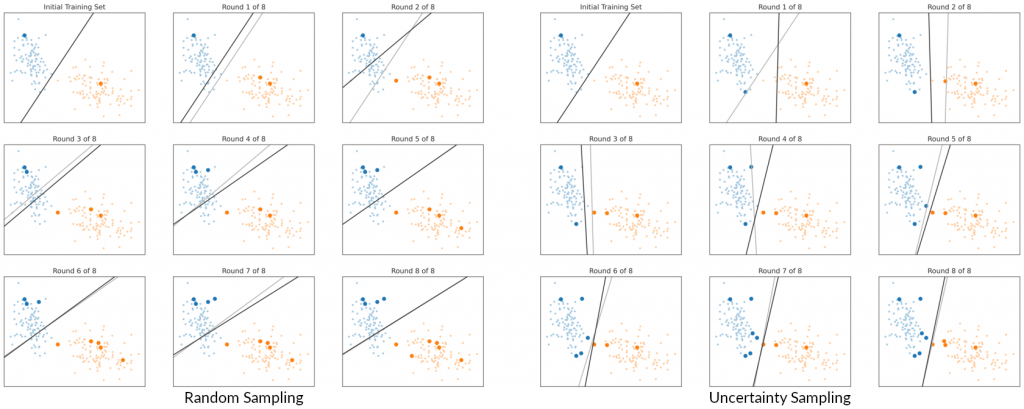
Before we begin, though, let’s look at a toy example that shows the benefits of Active Learning over random labeling. Here, the goal was to train a logistic regression classifier to separate two point clouds. In the left image, I randomly sampled and labeled 10 data points for training. As you can see, the fit is far from optimal, because of the location of the sampled training data with respect to the rest of the data. In the right image, I used Uncertainty Sampling (see below) to select training samples, which resulted in a much better model. In fact, we could have stopped after the 5th round and still gotten a better model than with random sampling. You can try this out yourself in this notebook. While this example is certainly far from reality (only two features and linearly separable data) and also cherry-picked, it illustrates the central promise of Active Learning: Better models with fewer labels.

Basic components of Active Learning
The above example hints at the four basic components of Active Learning: first, large set of unlabeled data \(\mathcal U\); second, a smaller (possibly initially empty) set of labeled data \(\mathcal L\); third, a learner that learns a model \(\hat y = h(\mathbf x)\) from \(\mathcal L\); and fourth, some process that generates true labels \(y = \omega(\mathbf x)\). This process is also known as the oracle and usually performed by a human, but it can also be implemented by a robot that conducts experiments or some other process that generates ground truth labels. Regardless, querying the oracle is assumed to be costly, so the learner must try their best to reduce the number of queries to it.
There are three scenarios in which Active Learning may take place: Query Synthesis, Selective Sampling and Pool-based Active Learning. In Query Synthesis, the learner learns a generative model from the labeled data and uses this model to generate a sample to query a label for. This synthetic example is then labeled by the oracle and added to the pool of labeled data. However, there is no guarantee that the query makes sense to the oracle. In the beginning, the generative model may not be good enough to capture the data and in later stages the learner will likely generate samples so close to the decision boundary that even the wisest of oracles will have trouble deciding the label. For this reason, Query Synthesis is mostly of academic interest.

Selective Sampling is more applicable in practice. Here, the learner again learns a model from \(\mathcal L\), though this time the model is discriminative. It is then given a previously unseen sample to classify. The learner decides to either process this sample on their own, or to query a label from the oracle. In the latter case, the labeled sample is added to the training data \(\mathcal L\) and the cycle begins anew. In this setting, the learner has some agency, but no control over what label is chosen from \(\mathcal U\). This scenario is most applicable for models that are already in production.

In Pool-based Active Learning, the learner has maximum agency: Instead of just deciding whether to query a label for a given data point or not, it can actively search the unlabeled data \(\mathcal U\) for interesting samples to give to the oracle. This setting is most suitable when you are bootstrapping a model, before it goes into production, or when you want to re-train a model with a batch of new data.
In either case, the key to making any of this work is a utility function \(u(\mathbf x)\) that assesses the benefit of the learner knowing the label for \(\mathbf x\). In Selective Sampling, the oracle is queried, if \(u(\mathbf x)\) exceeds some threshold. In Pool-based Active Learning, the learner selects the sample from \(\mathcal U\) that maximizes \(u(\mathbf x)\). The question, now, is how to implement this utility function.
Uncertainty Sampling
The most straightforward approach is to make the utility inversely proportional to the uncertainty of the model with respect to the sample. This approach is known as Uncertainty Sampling and will work with any model, provided it can assess its uncertainty of a prediction. For models that give an estimate of class probabilities \(\hat P(y|\mathbf x)\), we can use the probability estimate of the most probable class to measure uncertainty, i.e., \(u(\mathbf x) = 1 – \max_y \hat P(y|\mathbf x)\). This criterion is known as Least Confidence score, because it selects samples where the model is least confident about the class, because all classes are approximately equally likely.
These are not the only interesting samples, though: what about cases where all but two classes can be ruled out, but either class is (almost) equally likely? This leads to the Minimum Margin score \(u(\mathbf x) = \hat P(y_2^\star|\mathbf x) – \hat P(y_1^\star|\mathbf x)\), where \(y_1^\star\) and \(y_2^\star\) are the first and second most probable classes. This criterion will select similar samples as the Least Confidence score, but it will also select samples that lie close to the decision boundary between two classes.
A third criterion is derived from information theory and looks at the entropy of the class predictions, \(u(\mathbf x) = \mathbb E\left[ -\log \hat P(y|\mathbf x)\right]\). This Entropy score is best understood as a measure of the information our model would gain if it knew the label of the sample: the utility is low for samples where it is certain about the class label and large for samples where the model cannot decide between the classes. This is similar, but not the same as the Minimum Margin score, because here we look at all classes at once. The plot below shows the subtle differences between the scores in a three-class problem. In binary classification, however, all three measures are equivalent.

As formalized above, all these measures require an estimate of the class probability, which is not always available. Some models, like LDA, the SVM and deep learning give un-normalized prediction scores or confidence values that look like, but aren’t, probability estimates. Luckily, there are methods to derive probability estimates from such models, like probability calibration and conformal prediction. At least in binary classification, the least confidence and minimum margin scores can also be implemented by measuring the distance to the decision boundary. Still, these methods rely on only one model, which may be a bad fit for the data, or become stuck when the initial samples were bad.
Query by Committee
Query by Committee (QBC) takes inspiration from ensemble methods. Instead of just one classifier, it takes into account the decision of a committee \(\mathcal{C} = { h_1, \ldots, h_C }\) of classifiers \(h_i\). Each classifier has the same target classes, but a different underlying model or a different view on the data. A random forest is a well known example of such a committee: the underlying model is a decision tree, but each tree in the committee is trained on a different subset of the features.
How does that help us with judging the utility of an unlabeled sample? Simple: If the committee agrees on the class, there is no need to query the label. If, on the other hand, the committee is in disagreement, we need to ask the oracle for guidance. In other words: the committee disagreement about a sample is a proxy for its utility. But how can we measure disagreement? If the committee is comprised of many members, the class probability can be estimated by the fraction of votes \(V(y)\) for each class \(y\), i.e., \(\hat P(y|\mathbf x) \approx \frac{V(y)}{C}\). However, the number of classifiers \(C\) in the committee is often not large enough to get a reliable probability estimate. Still, the entropy measure from above can yield a good utility function and is known as Vote Entropy in this context:
\(\displaystyle u(\mathbf x) = – \sum_y \frac{V(y)}{C} \log \frac{V(y)}{C}\quad \text{where}\quad V(y) = |\{h_i | h_i(\mathbf x) = y\}|.\)
As a side note, Uncertainty Sampling with a random forest can be interpreted as Vote Entropy QBC with decision trees as base model.
If the committee members give probability estimates, this measure can also be implemented with a soft voting scheme, where the vote counts \(V(y)\) are replaced with the sum of probability estimates from each committee member, i.e.:
\(\displaystyle u(\mathbf x) = -\sum_y \overline{P}(y|\mathbf x) \log \overline{P}(y|\mathbf x)\quad \text{where}\quad \overline{P}(y|\mathbf x) = \sum_{h_i in \mathcal C}\frac{\hat P_i(y|\mathbf x)}{C}.\)
This measure is also known as Consensus Entropy. Another way to exploit the probability estimates is to compute the sum of Kullback Leibler Divergences between the committee members and the overall class probability estimate,
\(\displaystyle u(\mathbf x) = \sum_{h_i \in \mathcal C} D_{\text{KL}}(\hat P_i | \overline P)\quad \text{where}\quad D_{\text{KL}}(\hat P_i | \overline P) = \mathbb E_{y \sim \hat P_i}\left[\log \frac{\hat P_i(y | \mathbf x)}{\overline{P}(y | \mathbf x)}\right].\)
Note the subtle difference to Consensus entropy: Consensus entropy measures undecidedness in the ensemble, whereas here, we measure the mean disagreement of individual members against the consensus.
Expected Model Change
Uncertainty Sampling and QBC are conceptionally quite similar: you train a model (or an ensemble) and take the output for an unseen sample as a hint about it’s utility. However, doing so may often select samples close to the decision boundary that are not all that useful to learn useful structure of the data.
Expected Model Change (EMC) tries to tackle this problem by shifting the focus to the future. Instead of asking about the uncertainty of a prediction, we ask how much model would change if we knew the label of a sample. Interesting samples are those that will affect the model the most.
A straightforward implementation of EMC is to just train a model for each possible label and compare the old and new model. This is, of course, prohibitively expensive in general. However, there are methods that utilize the training algorithm to make this approach somewhat more tractable. In gradient-based methods, like Deep Learning, we can use the expected length of the training gradient as proxy for model change, i.e.,
\(\displaystyle u(\mathbf x) = \mathbb E_y\left[ \left\| \nabla \ell \left(h; \mathcal L \cup {(\mathbf x, y)} \right) \right\| \right] \approx \mathbb E_y\left[ \left\| \nabla \ell\left(h; {(\mathbf x, y)} \right) \right\| \right],\)
where \(\ell(h; \mathcal L)\) is the loss function and \(\mathcal L\) is the training set. The approximation comes from the realization that \(h\) is a fully trained model and from the i.i.d. assumption on the training data. This means that the only change in the gradient can come from the sample \(\mathbf x\) and we only have to evaluate the loss function for each \(\mathbf x\), but not for all training data in \(\mathcal L\).
Expected Error Reduction
Expected Error Reduction (EER) follows similar ideas as EMC, but again looks at the model output instead of the model itself and also takes the other data into account. In particular, a sample \(\mathbf x\) is considered useful, if we can expect that knowing the label will reduce the future error on unseen samples. With \(\hat{P^{\prime}}\) denoting the updated model trained with knowledge about \((\mathbf x, y)\) and \(\mathcal U\) denoting all unlabeled samples, this can be estimated using 0/1-loss:
\(\displaystyle u(\mathbf x) = \mathbb E_y \left[ \sum_{\mathbf x_u \in \mathcal U} \left(\max_{y^{\prime}} \hat{P^{\prime}}(y^{\prime}|\mathbf x_u)\right) \right].\)
As with expected model change, we have to retrain a model \(\hat{P^{\prime}}\) for each possible label of \(\mathbf x\), which becomes impracticable fast.
The cost can be somewhat mitigated by Variance Reduction. Without going into too much detail, the idea is to leverage a well-known result from statistical learning and decompose the model error into a data noise term, a model bias term and a model variance term. As the noise term only depends on the data and the bias is induced by the choice of model, any reduction in the error can only come from the variance term. Solutions are generally a bit more involved than what we have seen so far and out of scope of this blog post.
For details, see, e.g., Burr Settles seminal work on Active Learning. Note that EER is only applicable in Pool-based Active Learning, because we need access to all yet unlabeled data \(\mathcal U\).
Density Weighting
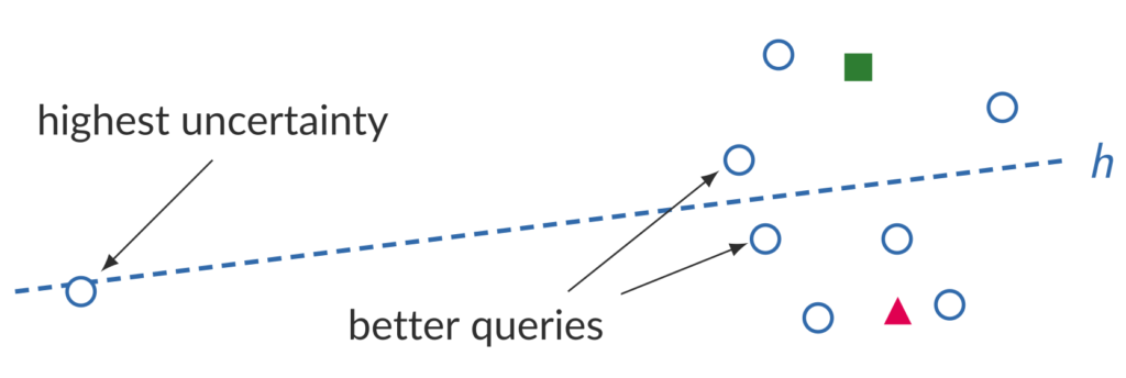
A big advantage of EER over Uncertainty Sampling and QBC is that EER takes all available data into account, while Uncertainty Sampling and QBC only look at individual samples. This myopic view of the data may lead to bad queries. For example, in the figure below, Uncertainty Sampling would query the label of the sample that is closest to the decision boundary, but clearly an outlier with respect to the rest of the data.

Density weighting mitigates this problem by weighting the utility \(u(\mathbf x)\) with an estimate of the density at \(\mathbf x\) to make sure that we do not sample queries in sparsely populated regions of the feature space, \(\displaystyle u'(\mathbf x) = u(\mathbf x) \hat p(\mathbf x)^\beta\). Here, \(u'(\mathbf x)\) is the modified sample utility, \(\hat p(\mathbf x)\) is the density estimate and \(\beta\) is a meta-parameter to control the strength of the density weighting. The density estimate can be based on a parametric model of the data or derived from a parameter-free method like kernel density estimation. In fact, it does not even have to be a true density, i.e., it does not need to integrate to 1 over the whole feature space, like the approach presented in Burr Settles survey.
Conclusion
If you have read this far: congratulations! You should now have an understanding of the fundamental ideas behind Active Learning and an overview of the basic techniques. Of course, we have barely scratched the surface; a blog post can only go so deep. For a more in-depth discussion, see Burr Settles Active Learning Literature Survey, which was the basis for this post, or his book on the topic. I also recommend Jens Röder’s dissertation Active Learning: New Approaches, and Industrial Applications, which presents an interesting approach based on distributional estimates of the posterior and contains even more references.
If you want to try out Active Learning in your projects, you should (like always) start small. Try out Uncertainty Sampling first, QBC second and bring out the big guns only if neither works for you. In this case it might also be worth to take a step back and think more deeply about the problem. Are there any other hints to help quantify the utility of a sample? Can you derive partial labels from metadata?
I also encourage you to take a shot at implementing these methods yourself. Uncertainty Sampling and QBC are not all that hard to implement yourself and even EMC is doable in a few lines of code. Have a look at the notebook that accompanies this blog post for inspiration. If you want to put Active Learning into production, however, it might be worth to check out the excellent ModAL Python package. ModAL features all of the strategies in this blog post (and more) and provides excellent documentation on top.


