
Notice:
This post is older than 5 years – the content might be outdated.
The amount of mobile applications making use of some sort of machine learning is quickly increasing, just as the number of potential use cases in this area. Whenever you chat with your virtual assistant about upcoming events or convert yourself into an avocado with a snapchat filter for your social media followers, you employ machine learning. The tools and frameworks jungle comprises more and more libraries to run those machine learning models directly on your mobile device, instead of sending the data back and forth to an inference server. One of those libraries is TensorFlow Lite, the successor of TensorFlow Mobile, of which you have probably read about in our older blog post. Indeed, this blog post series serves as a revised and extended rewrite of our article about TensorFlow Mobile and is divided into three parts. This first post tackles some of the theoretical background of on-device machine learning, including quantization and state-of-the-art model architectures. The second part deals with quantization-aware model training with the TensorFlow Object Detection API. The third part of this series describes how you can convert a model with the TensorFlow Lite model converter and how you can deploy the model using Android Studio.
If you are new to deep learning, I recommend you to first read our blog posts about Deep Learning Fundamentals and the concepts and methods of artificial neural networks before you move on with this post.
Why TensorFlow Lite?
TensorFlow Lite is a set of tools within the TensorFlow ecosystem to help developers run TensorFlow models on mobile, embedded, and IoT devices. It enables on-device machine learning inference with low latency and a small binary size. It comprises two main components, the TensorFlow Lite interpreter and the TensorFlow Lite converter. The former is used in the application to infer your optimized models on different platforms, including mobile phones, embedded Linux devices and microcontrollers. The TensorFlow converter converts the machine learning models into a format that can be understood by the interpreter. It also applies optimizations during the conversion process to improve performance and binary size of the model. With TensorFlow Lite, the machine learning models are inferred directly on the hardware, which comes along with some obvious advantages like reduced latency, since there is no network round-trip, increased privacy, because all data can stay on the device, and no need for an internet connection. Since TensorFlow Lite for Microcontrollers is still experimental, we will focus on TensorFlow Lite for mobile phones.
Basic concepts in mobile DL
Before we start building our TensorFlow Lite model, we will have a short look at some basic concepts and optimizations applied to machine learning models for use in mobile applications, including weight quantization and state-of-the art model architectures. The TensorFlow Lite interpreter currently supports a limited subset of TensorFlow operators that have been optimized for on-device use. This means that some models require additional steps to work with TensorFlow Lite. Thus, we will also have a look at the operators compatible with TensorFlow Lite. I will not provide a full list of all compatible operators here, especially since the amount of compatible operators increases with every release of TensorFlow Lite. If you want to build your own model and use it in a mobile application, have a look at the documentation on compatible operators.
Quantization
Machine Learning models are everywhere nowadays and it is crucial to run them efficiently, no matter whether you deploy them in the cloud or on the edge. For cloud deployment, you probably want to reduce latency or restrict the inference to only run on CPU because GPU servers are too expensive. Devices at the edge typically have lower computing capabilities and are constrained in memory and power consumption. Therefore, there is a pressing need for techniques to optimize models for reduced model size, faster inference and lower power consumption. One way to achieve this is to quantize the model either during the training process or afterwards.
Quantization refers to the process of reducing the number of bits that represent a number. In the context of deep learning, that means to reduce the information stored in each weight. It has been extensively demonstrated that weights and activations can be represented using 8-bit integers without incurring significant loss in accuracy. If you are interested in details on this topic, have a look at some papers with code on the task of quantization. Basically, the idea behind quantization is to map floating point numbers of infinital range onto fixed buckets of 8-bit integer values. Consequently, quantization is lossy by nature. For example, all floating point numbers between 1.5 and 1.8 will be mapped to the same integer representation, resulting in loss of precision. To mitigate this, TensorFlow also provides quantization-aware model training, which ensures that the forward pass computes the same result for training and inference, regardless of whether the weights are stored as floating point numbers or integers. This is achieved by adding fake quantization nodes to the graph in order to simulate the effect of quantization during forward and backward passes. These fake quantization nodes determine minimum and maximum values for activations during training. In other words, the fake quantization nodes are required to gather dynamic range information as a calibration for the quantization operation. Using this technique, a quantization loss is added to the optimizer as part of the overall loss. As a result, the model tries to learn parameters that are less prone to quantization errors. I created a colab notebook demonstrating quantization-aware training of an image classification model. If you want to get an in-depth look of quantization aware training in TensorFlow, I recommend reading the Google paper Quantization and Training of Neural Networks for Efficient Integer-Arithmetic-Only Inference.
State-of-the-art model architectures for mobile DL
Besides the optimizations that are applied to trained models in order to speed up inference, there are plenty of different model architectures that enable efficient CNN computation. At this point I have to mention that I am a computer vision guy, so this list deals with my personal affection for vision models.
MobileNet
The probably most known neural network architecture for mobile deep learning is MobileNet, whose latest version can be found here. MobileNet uses depthwise separable convolutions, which factorize a standard convolution into a depthwise convolution and a 1 × 1 convolution. Frankly, the depthwise convolution applies a single filter to each input channel and the 1 × 1 is used to combine the outputs of the former. Generally, it needs to be mentioned that not every kind of convolution is separable. Indeed, if we restrict ourselves to separable convolutions, we actually restrict the capabilities of our model. On the other hand, separating convolutions drastically reduces the amount of parameters and speeds up computation. The authors of MobileNet mention that by using 3 × 3 depth wise separable convolutions, they were able to reduce the number of parameters 8 to 9 times compared to standard convolutions. The following graphic illustrates the depthwise separable convolution in two steps.
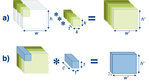
First, in step a), the depthwise convolution is applied to the input image of dimension w × h × c, where w is the width, h the height and c the number of input channels respectively. The kernel has different spatial dimensions, for example 3 × 3, but only one channel. Therefore we need c filters to retain the same shape for the output. Second, in step b, the newly generated feature maps are combined by a 1 × 1 × c filter to create a new feature of shape w’ × h’ × 1, which is the result of our depthwise separable convolution. Of course, the output shape can be altered by using multiple kernels in step b), e.g. if you use n kernels, the output shape will be w’ × h’ × n.
ShuffleNet
Another recent efficient CNN model is ShuffleNet. It combines the previously described depthwise separable convolution into group convolutions and adds a concept called channel shuffling. Group convolutions were first introduced in AlexNet to distribute the training to two GPUs. Group convolutions are not applied to all input channels, like a conventional convolution. Instead, we apply each convolution to a subset of the input channels. Imagine we have G groups, then each group g will be applied to Cin / G channels. Now, the problem is that we have to combine the output generated by the grouped convolutions, since if we don’t, our model will not learn any cross-group information. This would harm the overall performance of the network. ShuffleNet uses the channel shuffle operation to achieve exactly this. The output of one convolutional layer with G groups results in a G x n shaped feature map, where n is the number of channels per group. Before applying the next convolutions, this tensor is transposed and flattened, thus resulting in new subgroups being fed to the next layer. The graphic below visualizes this concept.
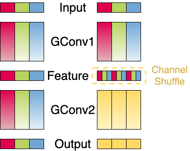
In the graphic, we have two stacked group convolutions (GConv) with three groups each, where each group consists of multiple channels. On the left, the second group convolution is applied to the output of the first group convolution and has the same amount of groups. As a result, the convolutions are applied to the exact same group as in GConv1, omitting information exchange across different groups. On the right, however, we apply the channel shuffle prior to the second group convolution. Mixing the output channels of the first group convolution, information of different groups is spread across all other groups for the second group convolution.
In combination with the grouped depthwise separable convolution, this forms a ShuffleNet Unit, which is displayed in the following graphic.
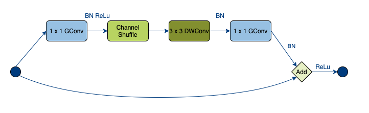
You can see that the architecture is inspired by ResNet which introduced this bottleneck unit style with residual connections.
EfficientNet
A recent branch of efficient CNN architectures embarks in the EfficientNet model family, which takes a completely different approach to the previously mentioned models. In its accompanying paper “EfficientNet: Rethinking Model Scaling for Convolutional Neural Networks“, the authors provide an insightful analysis of different model-scaling approaches, including width and height scaling, as well as image resolution scaling with respect to model performance. They introduce a new scaling strategy called compound scaling, which scales all three of the aforementioned dimensions in relation to each other by a user-specified coefficient. The intuition behind this strategy can be found in the following quote from the paper:
“We empirically observe that different scaling dimensions are not independent. Intuitively, for higher resolution images, we should increase network depth, such that the larger receptive fields can help capture similar features that include more pixels in bigger images. Correspondingly, we should also increase network width when resolution is higher, in order to capture more fine-grained patterns with more pixels in high resolution images.“
The compound scaling introduces four new hyperparameters, whereas each scaling dimension is associated with one hyperparameter and the fourth hyperparameter works as the compound coefficient to uniformly scale the three dimensions. The relationship of these parameters is shown in the following equation, where ϕ denotes the compound scaling factor, while ?, ? and ? specify how to assign the scaling to the network depth, width and resolution respectively.
depth: d = ?ϕ
width: w = ?ϕ
resolution: r = ?ϕ
s.t. ? · ?² · ?² ≈ 2
? ≥ 1, ? ≥ 1, ? ≥ 1
As a proof of concept, the authors evaluate their scaling strategy by applying it to the state-of-the-art CNN architectures MobileNet and ResNet. They complement their work by defining a new baseline architecture generated via neural architecture search. This baseline model, called EfficientNet-B0, is then used to incrementally build a whole model family by first applying a gridsearch to the parameters ?, ? and ? on the baseline network and later scaling the network up by altering the parameter ϕ with fixed ?, ? and ?. The authors show that EfficientNet outperforms the scaled versions of MobileNet and ResNet and reaches state-of-the-art results on different datasets while reducing the amount of parameters and FLOPS compared to recent other ConvNet architectures.
By the time of this writing we can find pretrained MobileNets and EfficientNets on TensorFlow Hub as ready-to-use modules.
Once-for-all Network (OFA)
A very recent approach to providing neural networks with efficient inference and competitive performance on limited hardware was presented at the International Conference on Learning Representations (ICLR) 2020 in the paper “Once-for-All: Train One Network and Specialize it for Efficient Deployment“. The authors describe a new approach to Neural Architecture Search (NAS), separating model training from the actual architecture search. This decomposition results in lower design cost (measured in GPU hours per training) and thus a smaller CO2 footprint than previous NAS techniques. While reading the section about EfficientNet above, you just learned about another NAS approach to design efficient neural networks that fit different hardware requirements by incorporating hardware feedback in the architecture search. However, given new inference hardware platforms, these methods need to repeat the architecture search process and retrain the model, resulting in rising GPU hours and cost. OFA takes a different approach. The main idea behind OFA is to jointly train a large network with many different sub-networks and later distill specific sub-networks for specific tasks.
Similar to EfficientNet, the architecture space of OFA comprises different layer configurations with respect to arbitrary number of layers, channels, kernel sizes and input sizes (in the paper denoted as elastic depth, width, kernel size and resolution, respectively). However, the training approach differs from compound scaling introduced in EfficientNet. OFAs are trained using progressive shrinking, which is meant to jointly train many sub-networks of different sizes, which prevents interference between the sub-networks. This is achieved by enforcing a training order from large sub-networks to small sub-networks for the elastic depth, width and kernel size dimensions, while keeping the resolution elastic throughout the whole training process by sampling different image sizes for each batch. As a result, smaller sub-networks share weights with larger ones. Let’s have a look at what this means for each of the scaled model dimensions:
- Elastic depth: To derive a small sub-network with only D layers from a larger network with N layers, OFA keeps the first D layers and skips the last N – D layers. Consequently, the weights of the first D layers are shared between small and large sub-networks. This is illustrated in the figure from the OFA paper below.

- Elastic width: Width corresponds to the number of channels per layer. The number of channels is reduced analogously to the number of layers. However, they are first sorted according to their importance with respect to the learning objective. The importance of a channel is measured as the L1 norm of its weights, while a larger L1 means more important. This is illustrated in the figure from the OFA paper below.

- Elastic kernel size: OFA supports kernel sizes of 7×7, 5×5 and 3×3. The smaller kernels can be merged into a large kernel while keeping the same center position. However, a problem with this approach is that the smaller sub-kernels may need to serve in different roles with different distributions or magnitudes. Kernel transformation matrices are introduced to compensate for this issue. This is illustrated in the figure from the OFA paper below.

Once the training is finished, we can derive a specialized sub-network that fits our deployment scenario. A deployment scenario comprises a combination of efficiency constraints, like latency or energy consumption while maintaining a high accuracy. As mentioned earlier, OFA decouples model training from architecture search. This is achieved by building neural-network-twins to predict latency and accuracy given a neural network architecture. Specifically, an accuracy predictor is trained on 16K randomly sampled sub-networks, whereas each sub-network is evaluated on 10K validation samples (in the paper this corresponds to ImageNet validation images). The accuracy predictor is a three layer feedforward neural network, which receives each layer of a sub-network and the input resolution encoded as one-hot-vectors with zero vectors for layers that are skipped. Alongside this accuracy predictor, a latency lookup table is used to derive the latency of a model on each target hardware platform. Given the target hardware constraint, an evolutionary NAS is performed on the neural-network-twins to derive the optimal sub-network.
The authors provide a PyTorch implementation of their approach on GitHub, as well as a nice Colab Notebook tutorial that demonstrated OFA on ImageNet. Unfortunately, by the time of this writing there is no existing TensorFlow implementation of OFA.
That is it with the theory for now. In the next part of this series, we will get our hands dirty and start with our model training using quantization-aware training with the TensorFlow Object Detection API. Stay tuned!


