Causal Inference: Introduction to Causal Effect Estimation

Recently, there has been a surge in interest in what is called Causal Inference. It is, however, not always clear what is meant by the term and what the respective methods can actually do. This post gives a high-level overview over the two major schools of Causal Inference and then dives deep into the basics of one of them. Along with this and another post on the topic (coming soon), we published the JustCause Framework, which intends to simplify the evaluation of causal effect estimation methods for researchers.

 What is Causal Inference?

To keep it short I will only briefly consider the wide field of Causal Inference and focus instead on a very specific problem setting: the estimation of treatment effects. If you’re familiar with the field, you can skip this section and jump right to the theoretical introduction below.

So, what is Causal Inference? Part of my thesis was to discern between the two major frameworks and corresponding names that are often brought up, when Causality is mentioned. One of them is Judea Pearl with his Structural Theory, the others are Neyman and Rubin and their Potential Outcomes Framework.

Pearl, after coming to fame in the community for his research on Bayesian Networks, started to study the power of graphs in modelling causal assumptions and drawing causal conclusions. His Structural Causal Models (SCMs) provide a wide range of clean mathematical tools to work with causation. In his own words, they aim to bridge the gap between how humans think about causal claims and how statistics expresses them. In his most recent work, The Book of Why, he argues that the implications of his research go far beyond the small community of researchers concerned with study design. Instead, he proclaims, his models help to formulate assumptions about all kinds of experiments and they help to make robust statements about what is possible and what is not. This stands in contrast to traditional statistics in the paradigm of Pearson and Dalton, which only speaks in probabilities and correlation.

To give an intuition without elaborating too much: SCMs can be used to model our assumptions about the effect of smoking on Asthma. We model all the causal relationships we know in the form of edges in a graph. Then, using deterministic algorithms, we can determine whether the effect we aim to isolate (namely, the effect of smoking on asthma) is identifiable using the data we have, say from a clinical survey. For the design and evaluation of studies in all sciences, this is revolutionary. But, to be clear, the tools of Pearl are only as good as the assumptions we feed them. And, unfortunately, it’s often these assumptions that are the hardest to come by. If you want to learn more about the field and how it can help to tackle a classic paradox of statistics (the Simpsons Paradox), consider reading the introductory chapter of my thesis, which elaborates on the topic in plain language.

The tools of Pearl are only as good as the assumptions we feed them. And, unfortunately, it’s often these assumptions that are the hardest to come by.

On a personal note I can only recommend looking at The Book of Why, even if you’re not directly confronted with causality. It sheds a much needed new light on statistics and introduces a new way of thinking about problems that is delightful and, as Pearl says, turns logical problems into playful games.

The Potential Outcomes framework, on the other hand, is (merely) a neat extension of traditional statistics into the realm of causality. Its merit lies in the fact that no new way of thinking is required. Instead, the known and proven tools of statistics can be applied. So let’s explore how this works.

Treatment Effects and Formal Notation

When studying treatment effects under the potential outcomes framework, we are interested in the effect a treatment \(T\) has on an individual, group or instance (called unit) \(i\) that has some features \(X_i = \{ x_{i1}, x_{i2}, … x_{id} \}\). Usually, we’re interested in the outcome \(Y_i\) depending if treatment was given or not. That is to say \(T_i \in \{ 0, 1 \}\). Thus there are two potential outcomes for each individual: \(Y_i(1)\) if \(i\) received treatment and \(Y_i(0)\) if it did not receive treatment or received a control/placebo.

It is obvious from this construction that in a realistic setting we can only ever see either \(Y_i(1)\) or \(Y_i(0)\) for any one unit and experiment.  This is why it is called the potential outcomes framework. Formally, we can write this mutually exclusive relationships as

\(Y_i = T_i \cdot Y_i(1) + (1- T_i) \cdot Y_i(0)\).

The treatment effect \(\tau\) is then defined as

\(\tau_i = Y_i(1) – Y_i(0)\).

We see here, that the quantity we are aiming to estimate is never observable, unlike in supervised machine learning, where we usually have ground truth for our data. To put it differently, causal analysis is the analysis of a fictional or counterfactual world. Because to estimate the treatment effect we are required to make statements about the counterfactual outcome that we did not observe. Since it introduces this so called super distribution, which contains factual and counterfactual distributions—and by assuming their validity—the potential outcomes framework can be seen as an extension of traditional statistics.

Causal Structure: Experiment vs. Observation

To better understand the difficulty of treatment effect estimation, let’s consider an example: Say we want to study the efficacy of Aspirin as a headache treatment. We can run a randomized control trial, which is the standard for modern drug research. That means we randomly give people either a placebo or the drug and we don’t tell them what they got. We then simply compare the outcomes (level of headache) for the people who did in fact get treatment and those who got a placebo. And because all that was done randomly we can be pretty sure that the result we get is the actual effect.

The idea is that by assigning treatment randomly and keeping participants in the dark, we remove all possible confounders. Confounders are things that influence both the treatment and the outcome. And by doing so, confounders water-down the significance of the measurements. To see why this is problematic, let us look at an observational trial.

In this case, instead of randomly assigning treatment, we just observe a population of people of which some choose to take Aspirin and some didn’t. If we now make the same comparison of outcomes between treated and control, the effect will be biased. This is because of confounders. Say, for example, people who took the aspirin did so, because they know that is important to look after themselves. Besides the aspirin, they also drank a lot of water and rested well. Now just from looking at the data, we cannot ever know whether their relief of headache is because of the aspirin or because they just rested. All we might see is a correlation between aspirin and headache, but we can’t be sure where that correlation came from. In Causal Graphs, a tool from Pearl, we can clearly see how the two settings differ.

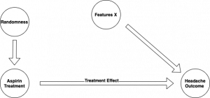
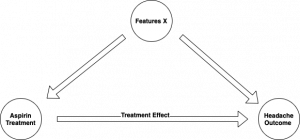
We can consider the edges in the graph as conveying statistical (correlational) information in both directions, while they only convey causal information in the direction they’re drawn. After all, if A causes B, then A is correlated to B, as well as the other way round (There is no statement about direction in statistics). Figuratively speaking, we can now see in the latter graph, that the correlation between headache and aspirin might not come from the treatment but rather from the longer path over the features. This is the idea of confounding, visualised in terms of Pearl.

The power of the treatment effect estimation method now lies in using observational and thus biased data (drawn from the latter of the two graphs) to make valid statements of clean treatment effects. That is to say, we use these methods to remove confounding bias from the data. Read on to learn how that is done.

How to estimate effects

Regression Adjustment

The simplest of all individual treatment effect approaches is, in my opinion, the Regression Adjustment using a single learner. Formally, we try to estimate the distribution of the expected value given features and treatment:

\(\mu(x, t) = \mathbb{E}[Y \mid X = x, T = t]\).

This is a straightforward regression task, where we use \(X\) and \(T\) as features/independent variables and \(Y\) as the dependent variable. If we use a linear regression, for example, and have 3 features plus treatment then the regression looks like:

\(\mu(x, t) = \alpha_1 x_1 + \alpha_2 x_2 + \alpha_3 x_3 + \beta t \cong \mathbb{E}[Y \mid X=x, T=t]\).

Now if the model assumption is true and the relationship between covariates and outcome is really linear, then the regression will return an unbiased estimate and we can get the unbiased treatment effect estimate

\(\hat{\tau}_i = \hat{\tau}(x_i) = \mu(x, 1) – \mu(x, 0)\).

And if we plug in the formula of the simplistic 3 feature example from before with linear regression this yields \(\hat{\tau}_i = \beta\).

In other words, the treatment effect is constant by definition, if we use a linear regression with the S-Learner. In some settings, however, the treatment effect does heavily depend on the features. It is said to be a heterogeneous treatment effect. By choosing say a RandomForestRegressor instead of a linear regression, we can overcome that drawback and still use the S-Learner principle.

The T-Learner works in a similar way, but it uses, as the name implies, two learners to do the same. One is only trained on treated instances, the other on control instances. I’ll explain in the article on campaign targeting how that works in more detail.

On a conceptual level, regression adjustment aims to simulate a control trial. By holding constant the feature values and only changing the treatment manually we simulate a counterfactual trial where the same individual get’s the opposite treatment. One can proof that already a simple S-Leaner will return the correct treatment effect, given the model assumption is true and there is enough data. (The estimate is unbiased, but variance depends on sample size.)

Tree Based Techniques: Covariate Balance

Another approach that has been very popular recently is based on decision trees and bears the iconic name Causal Forest. Because the mathematical formulation is rather unwieldy, I’ll stick to an informal introduction.

The idea with a causal tree as part of the causal forest is to split the covariate space into similarity leaves. The assumption is that within one leaf, instances are similar enough to compare the treated with the untreated as if they came from a randomised control trial. This means that instances within one leaf are similar except the fact that some are treated and some aren’t. How exactly this tree is built is non-trivial, as the true treatment effect of which we want to minimise the within-leaf variance, is not known. But by using smart reformulations of the problem, the authors of the original paper manage to derive a splitting criterion that yields provably consistent results. Also, they tackle the bad habit of trees to overfit on the training data with the so called honest property. 

The concept behind the causal trees is akin to that of covariate matching, where the idea is to match similar instances from both treatment groups. But instead of simply using a euclidian distance metric to find similar instances, the tree is used as an adaptive neighbourhood metric, which can deal with complex and high-dimensional relationships more easily.

An example study

To compare the two learners we’ve introduced above—and many others—I want to run a synthetic example study, which neatly highlights the strengths, weaknesses and differences of the methods.

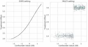
We use the 25 covariates/features of 747 instances out of the Infant Health Development Program (IHDP). Based on these, we generate synthetic outcomes and assign a confounded or biased treatment. Here you can see again in formulas what was visually represented in the graphs above. The feature \(X_8\) influences the treatment and the outcome. We generate the data here synthetically in order to have ground-truth, which is not available for real data.

Let’s say we define outcomes as

\(y_0 = \mathcal{N}(0, 0.2)\)

\(y_1 = y_0 + \tau\)

\(t = BERN[\sigma(X_8)] \)

and for \(\tau\) we define to variants: EXPO and MULTI. EXPO is defined simply as

\(\tau_e = \mathrm{exp}(1 + \sigma(X_8))\)

while MUTLI is defined explicitly as a multi-modal effect. Above, \(\mathcal{N}, BERN, \sigma\) are the normal distribution, the Bernoulli distribution and the sigmoid function respectively. That is to say, there is two groups within the dataset. One that reacts strongly to treatment and one that does react with a small effect only. Whether a patient is in group one or two depends strictly on feature \(X_8\). Let

\(\gamma = \mathbb{I}\left(\sigma(X_8) < 0.5\right)\)

\(\tau_m = \mathcal{N}(3 \cdot \gamma + (1-\gamma), 0.1)\),

where \(\mathbb{I}\) is an indicator function which yields 1 if the condition inside is true and 0 otherwise.

In the exponential setting, \(X_8\) is also the driving variable, but there is a smooth transition of effects from weak to strong. This is neatly visualised in the confounder plot below, where we plot the confounder against the treatment effect.

Method Comparison

With the DGPs above we now run a method comparison of a few basic learners. We compare, among others, an S- and T-Learner with Linear Regression and RandomForests and also a CausalForest. We do this using our framework JustCause, which was designed for exactly that purpose. All the code and more plots can be found in the notebook. (Clone the repo and run it yourself)

First, we load the data which are already implemented in JustCause. We sample 100 replications of the same data generating process in order to reduce sample variance and its influence on the metric.

Next we define the learners we want to use. We use the three shortly introduced above and also add the X-Learner in two variants using either Linear or RandomForestRegression.

Finally, we can run the evaluation of individual treatment effect (ITE) predictions using the metrics we desire on the EXPO synthetic data:

if we look only at the mean summary of the PEHE score over all replications, which is essentially a root mean squared error of individual treatment effects, we get:

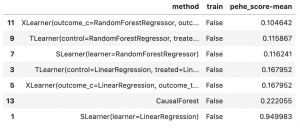
If we run the same evaluation on the MULTI setting, however, we get

Take a look at Chapter 5.3 of the thesis, if you’re interested in understanding, why linear learners are sometimes better suited than sophisticated CausalForests.

Take-Aways

All in all, I hope this article helped you grasp the field of Causal Inference a little better. I hope you now have a first understanding of what treatment effects are and why it is difficult and interesting to study them using machine learning methods. And lastly, I hope you’ve seen how simple it can be to run a basic evaluation using JustCause. 

If you are involved in the field, be it in research or practice, feel free to get in touch with us. We are welcoming new contributors to our just cause: making method comparison easier, less error prone and reproducible by design.