
TL;DR:
The Core Problem
Electricity demand is naturally hierarchical, spanning local, regional, and national scales. However, when forecasting models are developed for specific levels in isolation, the results are often incoherent: the sum of local forecasts does not match the national total. This inconsistency can lead to conflicting generation schedules and grid reliability risks.
Methodology & Experimental Setup
The data: Real hourly demand data from the US Energy Information Administration (EIA-930) was used. The system has a three-tier structure: 53 local grid operators form 13 regions, which in turn make up the entire US national grid.
The hierarchical forecasting process:
- Base forecasts: First, standard models (such as ARIMA or ETS) generate independent forecasts for each individual level (day-ahead forecast).
- Reconciliation: Since these forecasts do not match, they are mathematically “adjusted.“ A matrix ensures that the local figures ultimately add up exactly to the regional and national totals.
The endurance test: To test its reliability, the process was retested daily over an entire year (365 test runs) to cover all seasons and peak loads.
Key Findings
Correction does not save poor estimates: If the base model (such as ARIMA) makes gross errors at the local level, the reconciliation also “infects“ the higher levels. When using a stable base model (like ETS), reconciliation successfully enforces consistency without sacrificing accuracy, providing a “single source of truth“ for grid operators.
Imagine being responsible for forecasting electricity demand for the entire United States. Your national forecast affects grid stability planning and long-term infrastructure investments. At the same time, regional system operators and local utilities produce their own demand forecasts to plan generation schedules and manage congestion. Now imagine that the sum of these regional forecasts does not match the national projection. Suddenly, planning becomes inconsistent, coordination breaks down, and reliability risks emerge.
Situations like this are not hypothetical – they arise when forecasts are produced independently across different levels of an interconnected system. In the energy sector, where accurate and coherent demand forecasts are essential for reliable operation, such inconsistencies can have serious consequences.
This challenge is a prime example of a broader class of problems addressed by Hierarchical Time Series (HTS) forecasting. HTS consists of collections of time series linked through an inherent hierarchical structure, such as national, regional, and local electricity demand. While this structure is common in practice, it is often ignored during model development, leading to forecasts that are accurate in isolation but inconsistent across aggregation levels. By explicitly incorporating hierarchical relationships into the forecasting process, it becomes possible to ensure coherence throughout the system and, in many cases, improve forecast accuracy across aggregation levels. In this blog post, we explore the potential of hierarchical time series forecasting and demonstrate how leveraging this structure can meaningfully enhance electricity demand forecasting in the United States.
What Are Time Series?
Whenever data is observed sequentially over time, it forms a time series \(\{ y_t\}\), typically recorded at evenly spaced intervals \(t = 1, …, T\) such as hours, days, or months. In essence, a time series can be viewed as a stochastic process whose observed values combine an underlying signal and random noise. For a more detailed introduction to time series concepts, we refer the reader to this blog post on time series.
One of the central goals of time series analysis is forecasting: using historical observations to predict future values over a given forecast horizon. Formally, given \(T\) observed data points, we aim to predict future values \(\hat{y}_{T+h|T}\) for a forecast horizon \(h\). After fitting a model on past data (the training set), forecasts are evaluated by comparing predicted and observed values in future periods (the test set), with the difference between them referred to as the forecast error.
Forecasting techniques generally rely on the assumption that historical patterns persist and can be learned from past data. In time series settings, this means identifying underlying structures such as trends and seasonality while accounting for irregular fluctuations or random noise. What makes time series unique is that observations are not independent. Due to their temporal dependence, each observation is influenced by those that precede it. This feature poses challenges for traditional models, which often operate under the assumption that data points are independently and identically distributed (i.i.d). Consequently, these conventional models are not suitable for time series data.
Forecasting Models
Over the years, a wide range of forecasting models has been developed, each based on different assumptions about how information from the past influences the future. A simple but often surprisingly strong baseline is the persistence (naïve) model. It assumes that the most recent observation is the best predictor and sets all forecasts to the last observed value. A seasonal variant instead repeats the most recent seasonal cycle and is often effective for periodic data.
More flexible approaches relax this extreme assumption by allowing past observations to contribute with different importance. Exponential smoothing (ETS) models implement this idea by assigning exponentially decreasing weights to historical values and can capture level, trend, and seasonality in a unified framework.
Another widely used class of models is ARIMA, which models temporal structure through autoregressive terms moving-average components combined with differencing. ARIMA and ETS complement each other: one is based on autocorrelation structure, the other on trend–seasonality decomposition.
For a deep dive into forecasting for electricity consumption, we refer to this blog post where time series analysis with the prophet model is explored.
Time Series Are Often Hierarchical
Only a few real-life situations can be fully captured by a single time series. In most cases, multiple time series are observed instead, following a hierarchical structure across various levels. Lower-level series represent fine-grained measurements, while higher-level series represent aggregated totals. Two examples of such a hierarchy can be seen below.
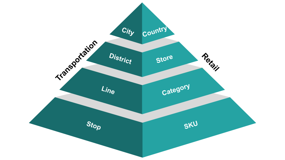
Hierarchical relationships in HTS are often formed through aggregation, but they can also arise from more general linear constraints.
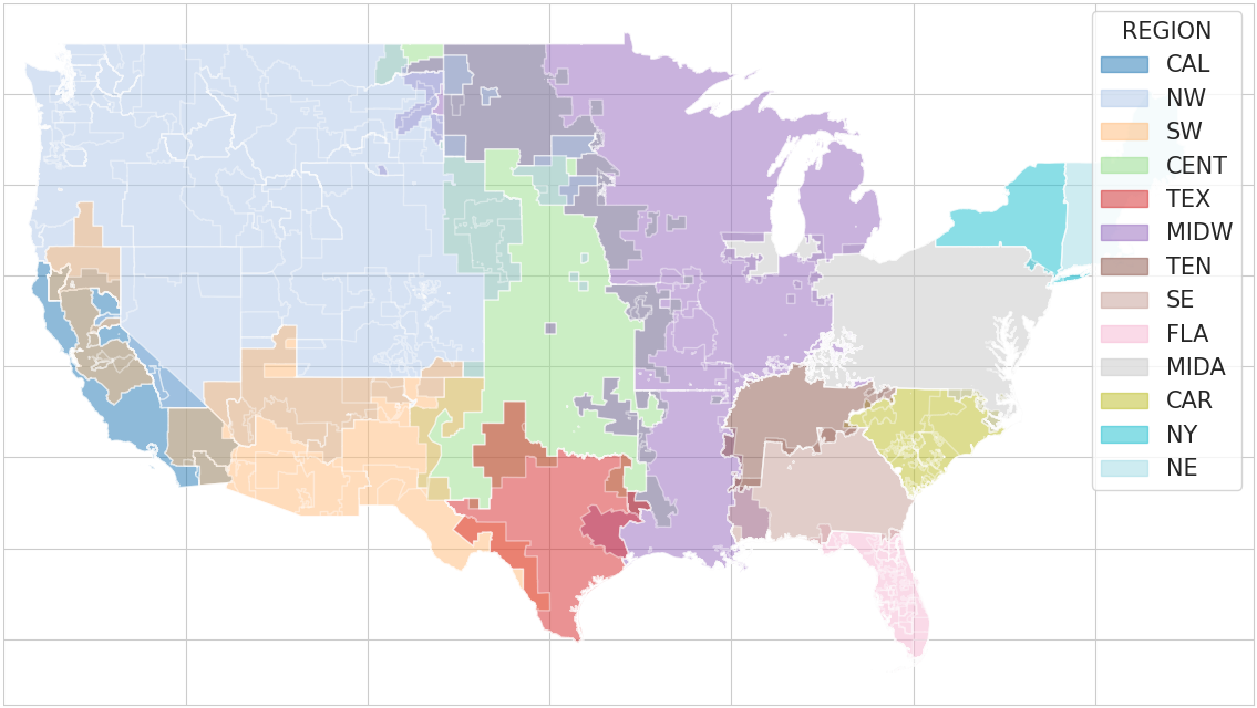
The electricity system of the United States naturally exhibits this structure. Electricity demand is measured and reported hourly at different levels of granularity. At the bottom of the hierarchy are the Balancing Authorities (BAs), each responsible for balancing supply and demand within its own area. These BAs are grouped into larger regions. At the top sits the continental U.S. total, which is simply the sum of all regions. The figure below provides a geographic overview of the regional groupings of BAs in the U.S. electricity system. The borders are overlapping due to shared responsibilities.
This multi-level structure can be expressed formally using a summing matrix \(\textbf{S}\), which maps the vector of bottom-level series \(b_t\) into the full set of series across all hierarchical levels: \[y_t = Sb_t.\] Here,
-
\(b_t\) contains BA-level demand,
-
\(y_t\) contains BA, regional, and national demand together,
-
and \(S\) encodes which BAs belong to which regions, and which regions aggregate to the total.
Simply speaking, the Matrix \(S\) describes the “blueprint“ of the power grid, which defines who belongs to whom. Moreover, this representation mirrors the physical reality of the grid: regional demand is literally the sum of its underlying BAs, and national demand is the sum of all regions.
The Coherence Problem
From a forecasting perspective, the hierarchical nature of electricity demand is more than a structural curiosity – it has direct operational consequences.
If we forecast each series independently – for example, forecasting demand for each BA and separately forecasting the regional and national total – there is no guarantee that these forecasts will align. For example, the sum of BA-level forecasts may seriously exceed the forecast for their region. This situation is known as incoherence. This inconsistency can cascade into practical issues: operational planning, market bidding, reliability studies, and resource allocation all depend on a consistent picture of future demand across grid layers.
This makes coherence an important goal when forecasting HTS. A set of forecasts is coherent if it obeys the same aggregation rules as the actual hierarchy by satisfying \[\hat{y}_{T+h \mid T} = S \hat{b}_{T+h \mid T}.\] In other words, coherent forecasts are those where forecasts at higher levels are exactly equal to the sum of the forecasts at lower levels.
Hence, our question is
- How can we find coherent forecasts and
- will coherence ideally also lead to an improved accuracy?
Leveraging the Hierarchy
Single-Level Approaches
The traditional and most intuitive approach for ensuring coherence when dealing with HTS is to generate forecasts for one level of the hierarchy and use those forecasts to obtain also forecasts for the other levels by linearly combining them.
 In the bottom-up approach, all bottom-level series are forecast independently and then aggregated to produce higher-level forecasts. This method preserves all information at the most granular level but can suffer from reduced accuracy if lower-level series are noisy.
The top-down approach takes the opposite route: a forecast is generated at the top level and then disaggregated to lower levels using predefined proportions. While this often yields stable higher-level forecasts, it may fail to capture dynamics at the lower levels.
The middle-out approach combines both ideas by forecasting at an intermediate level, aggregating upward and disaggregating downward. Although this can balance stability and granularity, it remains heuristic in nature.
These single-level approaches rely heavily on forecasts from one chosen level and do not fully exploit the information contained across the hierarchy. Early research focused on comparing these methods, with results showing that their relative performance depends strongly on data characteristics such as noise and cross-series correlation. This limitation motivates more systematic approaches that use information from all levels simultaneously.
Forecast Reconciliation
Forecast reconciliation takes a more principled approach. Instead of selecting one level to model, base forecasts are generated independently for every series in the hierarchy – bottom, intermediate, and top levels alike. These forecasts are generally incoherent and are subsequently adjusted to satisfy the aggregation constraints.
Let \(\hat{y}_{T+h|T}\) be the vector of all base forecasts across all levels. Reconciled forecasts are obtained as \[\tilde{y}_{T+h \mid T} = SG\hat{y}_{T+h \mid T}.\] where \(S\) represents the hierarchical structure and \(G\) is a reconciliation matrix that determines how information from different levels is combined. Simply speaking, we first generate independent forecasts for all time series, and then we mathematically “adjust“ them (by using \(G\)) until they fit together and satisfy the hierarchical constraints. Different choices of \(G\) lead to different reconciliation methods, with classical single-level approaches emerging as special cases.
Modern reconciliation methods estimate \(G\) using statistical properties of the base forecast errors, such as variances and covariances. This yields forecasts that are not only coherent but often more accurate. Prominent examples include Ordinary Least Squares (OLS), variance-scaled Weighted Least Squares (WLSv), structure-scaled Weighted Least Squares (WLSs), and Minimum Trace (MinTs) approaches, which differ in their assumptions about forecast error dependencies.
A more recent approach, ERM (Empirical Risk Minimization), formulates reconciliation as an empirical risk minimization problem, directly optimizing forecast accuracy and relaxing the assumption of unbiased base forecasts.
Forecast reconciliation is model-agnostic and can be applied as a post-processing step to any forecasting method, even when different models are used across series. By enforcing coherence and leveraging information from the entire hierarchy, reconciliation can improve overall accuracy, although gains at some levels may come at the expense of others.
Applying This to U.S. Electricity Demand
Which reconciliation method is best suited strongly depends on the specific use case, the dataset, and the underlying forecasting models. As a result, a big part of research is dedicated to evaluating the reconciliation methods across datasets that differ in the number of time series, domain, hierarchical depth, and the number of series per level.
Within the energy sector, HTS forecasting has been studied in a variety of contexts. Existing work often focuses on building-level data, smart meter measurements, and renewable generation such as wind and solar power. Electrical grid datasets have also been considered, but typically only for limited subsets of the system. To the best of our knowledge, the electricity demand of the entire U.S. grid has not yet been studied as a complete hierarchical system.
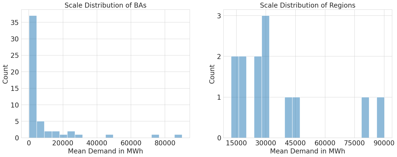
This use case introduces several challenges. The hierarchy is comparatively large, consisting of 53 BAs grouped into 13 regions. In addition, the scale of the time series varies strongly across BAs (as can be seen in the following graphic), making it difficult to capture local patterns that can easily be overshadowed by larger-scale series. Finally, BAs are unevenly distributed across regions, which further increases the structural complexity of the hierarchy.
Data Set
We use the publicly available EIA-930 dataset, published by the U.S. Energy Information Administration (EIA). The dataset provides high-frequency insight into electricity system operations across the contiguous United States. Every hour, each BA reports its demand, net generation, and interchange values directly to the EIA, making it one of the most granular sources of grid data available.
For this analysis, we focus exclusively on electricity demand, and therefore exclude BAs that report only generation or interchange. Additionally, we also remove inactive BAs and impute remaining missing values to ensure that the hierarchy is complete across all levels and timestamps. This yields a clean, consistent dataset of hourly demand at the BA, regional, and national levels.
Experimentation Setup
The aim of our experiments is not to identify the best possible forecasting model, but to compare how different reconciliation methods behave on real U.S. electricity demand data. Consequently, the base forecasting models – ETS and ARIMA – are fit using analytical procedures without any hyperparameter tuning. This avoids modeler-induced bias, since no subjective adjustments are made after inspecting the results, and eliminates the need for a dedicated validation set. We therefore evaluate the performance using a straightforward train–test structure.
To reflect operational practice, we forecast 24 hours ahead, aligning with the day-ahead commitment decisions that BAs must make. Model performance is evaluated using a time-dependent cross-validation with 365 rolling iterations, corresponding to each day of the year. Each iteration produces a new 24-hour-ahead forecast based on an updated training window, providing a diverse set of evaluation scenarios across different seasons, demand conditions, and grid states. This design ensures a robust assessment of reconciliation performance over time.
In our experiment, we compare a broad set of reconciliation approaches applied to two base models (ETS and ARIMA) with a coherent baseline – the seasonal naive model. We include the classical single-level strategies (Bottom-Up, Top-Down, and Middle-Out) and, after testing multiple disaggregation rules, use forecast-proportion disaggregation due to its consistently strong results. Among the statistically grounded methods, we evaluate OLS, WLSs, WLSv, MinTs, and ERM. Reconciliation is applied at each cross-validation step to ensure that all methods operate under identical forecasting conditions. Performance is measured using standard metrics such as Mean Absolute Error (MAE), Root Mean Square Error (RMSE), and Mean Absolute Scaled Error (MASE), with results reported at all levels of the hierarchy (BAs, regions, and national).
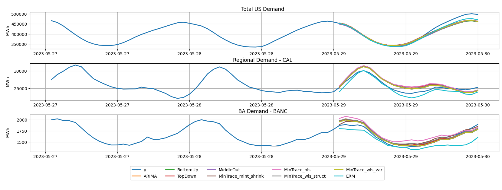
The figure below illustrates a single cross-validation split for the Balancing Authority of Northern California (BANC), which belongs to the California (CAL) region, shown across three hierarchy levels: national (top), regional (middle), and BA-level (bottom). The solid blue line represents the observed electricity demand, while the orange line shows the incoherent base forecast produced independently at each level. The remaining lines correspond to different reconciliation methods, all of which enforce coherence across the hierarchy. In this specific example, ERM tracks the observed demand more closely at the regional level than several alternatives, whereas at the BA level, its forecast deviates slightly more from the observations. This highlights how reconciliation can redistribute forecast accuracy across hierarchy levels rather than uniformly improving performance everywhere. Importantly, this figure is intended as an illustrative example for a single BA and cross-validation split. To assess whether these patterns persist more generally, we next examine results aggregated across the full experimental evaluation.
 Results
We now evaluate the performance of ARIMA, ETS, and their respective reconciliation methods. Although multiple error metrics were considered during cross-validation, we focus here on MASE for clarity, as its scale independence allows meaningful comparisons across hierarchy levels.
A central takeaway from the experiments is that reconciliation does not rescue a weak base model. Instead, its effectiveness depends critically on the quality and stability of the underlying forecasts.
ARIMA-based forecasts: when complexity backfires
Despite its flexibility, ARIMA performs poorly at the BA level, exhibiting very large errors across all metrics. These errors are driven by a small number of extreme forecast failures, which heavily distort average performance. At the regional and national levels, ARIMA fails to outperform the simple SeasonalNaive baseline.
Reconciliation does little to alleviate this problem. In fact, several reconciliation methods amplify ARIMA’s weaknesses. Bottom-Up reconciliation propagates the severe BA-level errors directly to higher levels, leading to consistently poor performance across the hierarchy.
While ERM substantially reduces error at the BA level, this improvement comes at the expense of worse regional and national forecasts, illustrating the redistribution of accuracy induced by reconciliation. Middle-Out and Top-Down perform best among ARIMA-based approaches, largely because they bypass the unreliable BA-level forecasts. Middle-Out even improves national-level accuracy. Nevertheless, neither ARIMA nor any of its reconciliation variants consistently outperforms the SeasonalNaive baseline.
In this setting, model sophistication proves to be a liability rather than an advantage.
ETS-based forecasts: robustness over complexity
The picture changes markedly when using ETS as the base forecasting model. Even without reconciliation, ETS delivers robust and reliable forecasts, outperforming SeasonalNaive at the BA and national levels while achieving comparable performance at the regional level.
With ETS as a base model, reconciliation methods become effective rather than harmful. Most ETS-based reconciliation methods perform at least as well as the SeasonalNaive baseline, and several yield improvements at specific hierarchy levels. In particular, Bottom-Up and WLSv reduce errors at the regional level while maintaining stable performance elsewhere. In these cases, reconciliation successfully leverages hierarchical information without disrupting already well-calibrated forecasts.
Not all methods benefit equally from this stability. Middle-Out, Top-Down, and WLSs fail to deliver improvements and even reduce accuracy at some levels, indicating that more aggressive or structurally driven adjustments can be counterproductive when base forecasts are already reliable. ERM performs worst in this setting, increasing errors across all hierarchy levels and highlighting that its bias–variance trade-off is poorly suited when little correction is needed.
OLS and MinTs illustrate the central tension of reconciliation: improvements at certain levels are accompanied by deteriorations at others. However, when considering all error metrics jointly, MinTs emerges as the most reliable performer. While it does not dominate at every single level, it consistently offers the best compromise across the hierarchy, balancing improvements and losses in a stable and predictable way.
Average MASE over all cross-validation steps by model and level:
| MODEL | BA | REGION | TOTAL | OVERALL |
|---|---|---|---|---|
| SeasonalNaive | 0.99 | 0.97 | 0.96 | 0.99 |
| ETS | 0.97 | 0.97 | 0.94 | 0.97 |
| ETS/BottomUp | 0.97 | 0.96 | 0.94 | 0.97 |
| ETS/MiddleOut | 0.98 | 0.97 | 0.95 | 0.98 |
| ETS/TopDown | 0.99 | 0.97 | 0.94 | 0.98 |
| ETS/OLS | 1.52 | 0.98 | 0.93 | 1.41 |
| ETS/WLSs | 1.22 | 0.97 | 0.94 | 1.17 |
| ETS/WLSv | 0.97 | 0.96 | 0.94 | 0.97 |
| ETS/MinTs | 0.97 | 0.96 | 0.95 | 0.97 |
| ETS/ERM | 2.27 | 1.45 | 1.16 | 2.09 |
| ARIMA | 28646.53 | 0.98 | 0.98 | 22660.89 |
| ARIMA/BottomUp | 28646.53 | 11636.82 | 11819.47 | 25094.99 |
| ARIMA/MiddleOut | 2.38 | 0.98 | 0.95 | 2.08 |
| ARIMA/TopDown | 2.39 | 1.00 | 0.98 | 2.10 |
| ARIMA/OLS | 130414.11 | 1090.42 | 68.16 | 103375.99 |
| ARIMA/WLSs | 94325.68 | 6605.17 | 3940.38 | 75956.25 |
| ARIMA/WLSv | 20013.46 | 2530.53 | 584.36 | 16331.27 |
| ARIMA/MinTs | 26473.41 | 15965.26 | 2095.76 | 24070.67 |
| ARIMA/ERM | 28.40 | 28.21 | 32.16 | 28.42 |
The bigger picture
Taken together, these results tell a clear story. Reconciliation cannot compensate for fundamentally unstable base forecasts, as illustrated by ARIMA’s failure at the BA level. When base forecasts are unreliable at the most granular level, reconciliation may propagate these errors through the hierarchy rather than correct them.
In contrast, when paired with a robust base model such as ETS, reconciliation becomes a powerful tool that enforces consistency while yielding favorable accuracy trade-offs across hierarchy levels.
Conclusion
The results of this study show that hierarchical forecasting is not just a modeling refinement, but an operational necessity for managing complex, multi-level electricity systems. By explicitly incorporating hierarchical structure, forecasts can be made internally consistent while leveraging information across aggregation levels.
From an operational perspective, coherent forecasts provide a shared and reliable view of future demand across the system. They ensure that local, regional, and national demand projections align, reducing contradictions between planning layers. This directly supports:
- more reliable unit commitment and dispatch decisions,
- improved market bidding strategies through consistent demand expectations,
- more efficient allocation of reserves and transmission capacity,
- and clearer communication between system operators at different levels.
Among the reconciliation methods considered, MinTs emerges as the most dependable approach. Rather than optimizing accuracy at a single hierarchy level, it acts as a stable mediator across the system, balancing forecast accuracy in a predictable way while preserving coherence throughout the hierarchy. This makes it particularly well suited for operational settings, where robustness and consistency often matter more than isolated performance gains.
Overall, this work shows that organizations managing hierarchically structured demand can benefit substantially from reconciliation-based forecasting pipelines. By combining robust forecasting models with statistically grounded reconciliation, operators can obtain forecasts that are internally consistent and, in many cases, more accurate – supporting better planning decisions, more efficient resource utilization, and ultimately a more reliable power system. These capabilities are key ingredients for operating modern, data-driven electricity systems.
Sources
B. J. Dangerfield and J. S. Morris. “Top-down or bottom-up: Aggregate versus disaggregate extrapolations“. In: International Journal of Forecasting 8.2 (Oct. 1992), pp. 233–241.
Delivery to consumers – U.S. Energy Information Administration (EIA). Url: https://www.eia.gov/energyexplained/electricity/delivery-to-consumers.php (visited on 01/27/2025).
E. S. Gardner and E. Mckenzie. “Forecasting Trends in Time Series“. In: Management Science 31.10 (Oct. 1985), pp. 1237–1246.
G. Athanasopoulos et al. “Hierarchical Forecasting“. In: Macroeconomic Forecasting in the Era of Big Data. Ed. by P. Fuleky. Vol. 52. Series Title: Advanced Studies in Theoretical and Applied Econometrics. Cham: Springer International Publishing, 2020, pp. 689–719.
G. Athanasopoulos, R. A. Ahmed, and R. J. Hyndman. “Hierarchical forecasts for Australian domestic tourism“. In: International Journal of Forecasting 25.1 (Jan. 2009), pp. 146–166.
G. Athanasopoulos et al. “Forecast reconciliation: A review“. In: International Journal of Forecasting 40.2 (Apr. 2024), pp. 430–456.
Real-time Operating Grid – U.S. Energy Information Administration (EIA). Url: https://www.eia.gov/electricity/gridmonitor/index.php (visited on 02/07/2025).
R. H. Shumway and D. S. Stoffer. Time Series Analysis and Its Applications: With R Examples. Springer Texts in Statistics. Cham: Springer International Publishing, 2017.
R. J. Hyndman and G. Athanasopoulos. Forecasting: principles and practice. Third print edition. Melbourne, Australia: Otexts, Online Open-Access Textbooks, 2021. 440 pp.
S. L. Wickramasuriya, G. Athanasopoulos, and R. J. Hyndman. “Optimal Forecast Reconciliation for Hierarchical and Grouped Time Series Through Trace Minimization“. In: Journal of the American Statistical Association 114.526 (Apr. 3, 2019), pp. 804–819.
S. Ben Taieb and B. Koo. “Regularized Regression for Hierarchical Forecasting Without Unbiasedness Conditions“. In: Proceedings of the 25th ACM SIGKDD International Conference on Knowledge Discovery & Data Mining. July 25, 2019, pp. 1337–1347.
S. H. Huddleston, J. H. Porter, and D. E. Brown. “Improving forecasts for noisy geographic time series“. In: Journal of Business Research 68.8 (Aug. 2015), pp. 1810–1818.
X. Wang, R. J. Hyndman, and S. L. Wickramasuriya. “Optimal forecast reconciliation with time series selection“. In: European Journal of Operational Research (Dec. 2024).