Machine Learning Interpretability: Do You Know What Your Model Is Doing?

Machine learning has a great potential to improve data products and business processes. It is used to propose products and news articles that we might be interested in as well as to steer autonomous vehicles and to challenge human experts in non-trivial games. Although machine learning models perform extraordinary well in solving those tasks, we need to be aware of the latent risks that arise through inadvertently encoding bias, responsible for discriminating individuals and strengthening preconceptions, or mistakenly taking random correlation for causation. In her book „Weapons of Math Destruction“, Cathy O’Neil even went so far as to say that improvident use of algorithms can perpetuate inequality and threaten democracy. Filter bubbles, racist chat bots, and foolable face detection are prominent examples of malicious outcomes of learning algorithms. With great power comes great responsibility—wise words that every practitioner should keep in mind.

With the adoption of GDPR, there are now EU-wide regulations concerning automated individual decision-making and profiling (Art. 22, also termed „right to explanation“), engaging companies to give individuals information about processing, to introduce ways for them to request intervention and to even carry out regular checks to make sure that the systems are working as intended. Recent research in computational ethics propose to raise awareness to optimization criteria like fairness, safety (2) and transparency when developing machine learning models. However, unlike usual performance metrics, these constraints are much harder if not impossible to quantify. Nevertheless, designing decision systems that are understandable not only for their creators, but also for their customers and users, is key to achieving trust and acceptance in the mainstream.

The Problem with Blackboxes

In recent years, ever falling cost of memory allows companies to collect huge amounts of data, while the evolution of distributed systems enables data processing at large scale. Consequently, with the (re-)emergence of deep learning and the maturity of dedicated machine learning frameworks, we are now able to tackle complex non-linear problems within high dimensional domains like NLP or computer vision. The underlying models are usually quite complex in terms of structure, containing a huge number of parameters to optimize across several interaction layers. In the following, these types of models are referred to as blackboxes, since humans are not able to explain their behaviour by simply looking at their internals.

The problem with blackboxes is the lack of trust caused by their opaque nature. A decision system should be doing the right thing in the right way but we are usually not able to guarantee that a certain prediction is derived in a way that it should have been. Consequently, it is hard to predict the models‘ future behaviour and to fix it in a targeted way in case of failure. The Dog-or-Wolf-classifier, described by Ribeiro et al., which turned out to be nothing else but a snow detector on steroids, is an illustrative example of a model that, despite of its predictive power, is not aligned with its problem domain. Furthermore, even seemingly robust classifiers are fooled by adversarial examples which are synthetic instances like generated images that are optical illusions to the algorithm.

Interpretability and Explanation Techniques

Interpretability in the context of machine learning describes the process of revealing causes of predictions and explaining a derived decision in a way that is understandable to humans. The ability to understand the causes that lead to a certain prediction enables data scientists to ensure that a model is consistent to the domain knowledge of an expert. An intuitive definition of interpretability in the context of machine learning is provided by Been Kim and Finale Doshi-Velez in „Towards A Rigorous Science of Interpretable Machine Learning“, where they describe it as the ability to explain or to present [a models decision process] in understandable terms to a human. This usually means at least identifying the most relevant features and their kind of influence (e.g. linear, monotone, etc.) to the models‘ predictions. In the context of machine learning, we can think of explanations as vehicles that facilitate interpretability.

Predictive models can roughly be distinguished between intrinsically interpretable models and non-interpretable „blackbox“ models. Intrinsically interpretable models are known to be easy for humans to understand. An example of an interpretable model is a decision tree, since it exhibits an intuitive, rule-based decision process. In contrast to that, neural networks can be classified as blackboxes due to their complex internal structure, which is tremendously harder for humans to grasp. Having said that, the distinction between interpretable and non-interpretable models is not obvious. Interpretable models are usually simple and somehow self-describing, showing moderate predictive performance. On the other hand, blackbox models have much better accuracy at the cost of comprehensibility. This is the reason why a trade-off between accuracy and interpretability has to be made in many cases.

There are basically two practices to approach interpretability:

1. Use intrinsically interpretable models
2. Apply post-hoc interpretability techniques to an existing model

The first approach is restricted to certain types of rather simplistic, mostly linear or rule-based models or to models that meet specific constraints regarding sparsity or monotonicity. It is widely adopted in the industry, but it leads data scientists to applying over-simplistic models to complex tasks. Furthermore, even models that are known to be easy for humans to understand can become vastly complex. Think about a linear model that relies on heavily engineered features or a deep and widely nested decision tree. To read more about criticism and misconceptions about interpretability, see Zachary C. Liptons comprehensive recap about „The Mythos of Model Interpretability“.

The second approach is more flexible since it is applicable to any model. Post-hoc techniques attempt to disaggregate a models predictions in order to identify the main drivers of its decision process. This is usually achieved by varying the input and evaluating changes in the output. The downside of post-hoc techniques is the increased complexity of the prototyping workflow. Furthermore, most interpretability techniques are approximate, hence providing potentially unstable estimates of explanations.

Post-hoc interpretability techniques can be further divided into techniques with a global scope and techniques with a local scope. Global techniques attempt to explain the entire model behaviour. In contrast to that, local techniques explain single predictions or the models behaviour within a closed region. The following table summarizes several post-hoc techniques along with their respective categories:

	Global	Local
Model-specific	Model Internals Intrinsic Feature Importance	Rule Sets (tree structure)
Model-agnostic	Partial Dependence Plots Permutation-based Feature Importance Global Surrogate Models	Individual Conditional Expectations Local Surrogate Models

Model internals refer to a self-describing structure of an interpretable model, like a decision tree or a linear model. Intrinsic feature importance estimates are usually calculated based on a specific model structure. This can be done by weighting split variables of a tree ensemble or comparing coefficients of a linear model. Model-agnostic techniques are especially useful when dealing with more complex models. In the following, I’ll apply some rather basic yet powerful techniques to explain a blackbox model.

Explaining a Blackbox Model

In the following, we will create a blackbox model to solve a regression task and explain its behaviour by applying post-hoc interpretability techniques. We will use the iml package which provides many tools to explain blackbox models in combination with the mlr package which provides a comprehensive and unified interface for prototyping. Both packages work seamlessly together and support many classification and regression models, e.g. random forests, neural networks, or GBMs.

Data Import and Analysis

Let’s first import all relevant libraries:

We will use the popular Boston Housing dataset which is also used in the iml tutorial. The dataset contains housing data for 506 census tracts of Boston from the 1970 census. Each record describes a district of the city of Boston with features like the per capita crime rate by town (crim), the average number of rooms per dwelling (rm) and the nitric oxides concentration (nox). The variable we want to predict is the median house value (medv) of a particular district. It is basically a supervised regression task based on tabular data containing a reasonable number of features. The authors of the tutorial have chosen a random forest approach to predict the target variable. In contrast to that, we will try a Kernel-based SVM.

Let’s import the data and do some basic analysis:

The dataset contains 506 records, 12 numerical features, a categorical feature (chas) and the target variable (medv). Fortunately, there are no missing values or extreme outliers. The median house value ranges from 5,000 USD to 50,000 USD, showing most values between 15,000 USD and 25,000 USD. There is a small peak at the maximum which could be caused by setting an upper limit at 50,000 USD.

Data Modelling

We want to predict the median house value using a SVM based on a Gaussian Radial Basis Function (RBF). For this approach, there are basically two hyperparameters to tune:

• C: the cost of constraints violation, which weights regularization
• sigma: the inverse kernel width for the Gaussian RBF

Let’s perform a repeated 10-fold cross validation for each parameter set of a parameter grid in order to get appropriate values for these hyperparameters:

Having determined appropriate hyperparameters, let’s fit the final model to the entire dataset:

Interpretation

The SVM we have trained in the previous steps performs quite well in solving the regression task. Unfortunately, we are not able to explain it because of its complex structure. In these situations, model-agnostic techniques are helpful since they can be applied to any model. In this section, we will apply some rather basic, yet powerful approaches to explain the overall behaviour of the model.

As a preliminary step, we will wrap the model along with its data in a Predictor object:

Feature Importance

At first, we will estimate the importance of each feature by evaluating their influence on the model’s performance. The importance of a feature is determined by repeatedly permuting its values and measuring the degradance of the performance measured by a certain loss function, e.g. mean squared error for this regression task. A feature is assumed to be important if the error significantly increases after a shuffle. In contrast to that, we assume that a permutation of a feature that is not important will not worsen the performance.

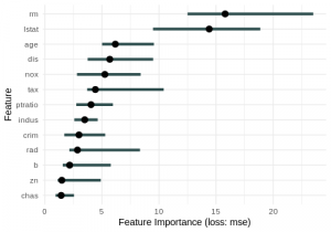
In the feature importance plot above, we see that two features rm (average number of rooms per dwelling) and lstat (percentage of lower status of the population) contribute by far the most to the model’s overall performance. Shuffling these features caused the MSE of the model to increase by an amount of around 15 on average (almost 4,000 USD). All other features caused the MSE to increase less than 7 on average which is still an error of 2,600 USD on average.

The advantage of this approach is that it produces a global, aggregated insight which is comparable across several types of models. Unfortunately, it is tied to a certain loss function, computationally intense and not applicable to high dimensional problems like NLP or computer vision.

Feature Effects

Now that we know which features are relevant, let’s determine how they influence the predictions by generating partial dependence plots (PDP) and individual conditional expectation curves (ICE). ICE curves show the dependence of the response on a feature per instance. An ICE curve is generated by varying the value of a single feature for a given instance, keeping the others fixed, and applying the model to the modified instance. This process is repeated so that an ICE curve is created for every instance of the dataset. We can draw conclusions about the overall marginal impact of a feature by looking at the PDP curve, which is generated by taking the point-wise average of the underlying ICE curves.

The following plots show the combined Partial Dependence (yellow) and ICE curves (black) for the most important features rm and lstat, centered at 0:

We see a relative consistent pattern in the ICE curves of both features. Any irregularities indicate dependency among features (see multicollinearity) since contradicting trends in ICE curves cannot be explained by variation of a single feature alone. Generating a PDP curve based on inconsistent ICE curves could be misleading and therefore should be avoided. This is the reason why PDP curves are based on the assumption of independence.

We further see a monotonic increase on average of the predicted median house value when increasing rm (the average number of rooms per dwelling) and a monotonic decrease on average when increasing lstat (percentage of lower status of the population).

Interaction Strength

Now that we identified the most relevant features rm and lstat along with their kind of influence, let’s take the other features into account by measuring how strongly they interact with each other. This is estimated by the H-statistic which measures the amount of variation of the response that is caused by interactions. Its value will be greater than zero for a given feature if interactions with any of the other features are relevant to the model. If a particular feature is completely independent of any other feature, the value will be zero.

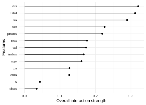
We see that ‚dis‘ (weighted distances to five Boston employment centres) shows the highest overall interaction strength of approximately 0.3. In other words, 30 % of the variation of the predicted median house value caused by feature ‚dis‘ can be attributed to interactions with other features. This sounds reasonable since distance to employment centres alone is not that meaningful to the median house value. When taking other relevant features like ‚lstat‘ or ‚crim‘ into account, distance to employment centres becomes more expressive. On the other side, ‚crim‘, the per capita crime rate by town, is relatively independent compared to other features.

Let’s also take a look at the 2-way interactions of the most important features:

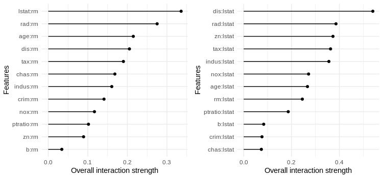
We see that the interactions between ‚rm‘ and ‚lstat‘ as well as between ‚lstat‘ and ‚dis‘ are most influential to the models predictions. What is also interesting is that interactions with ‚rad‘, the accessibility to radial highways, is quite expressive. Even if that feature was not determined as one of the most relevant features.

Global Surrogate

The last technique I want to demonstrate in this demo is the Global Surrogate. The idea behind it is to approximate a complex model by a simpler model and to draw conclusions about its behaviour by looking at the structure of the simple model. In our case, the simple model will be a decision tree of depth 2. We will fit it to the original features and the outcome of the blackbox model (not the original target variable!). The following plot shows the distribution of the predicted house values for each of the terminal nodes:

We see that lstat and rm were selected as the main split criteria, which is consistent to the feature importance estimate above. The distributions of the predicted outcome within the terminal nodes are significantly different, so the splits seem to be appropriate. The simple tree surrogate seem to capture the overall model’s behaviour quite well.

Conclusion

While performance metrics are crucial to evaluate a model, they lack explanations. In the vast majority of real-world tasks, it is impossible to capture every considerable aspect in a single numeric quantity to optimize for. The consequence that arises from this is that one cannot be sure that a model provides sound decisions and behaves in an acceptable and predictable way. To address this issue, the prototyping workflow can be complemented by Interpretability techniques in order to understand a model’s decision process. Furthermore, interpretability facilitates targeted debugging, since issues that arise from information leakage, multicollinearity or random correlations can be identified (just to name a few). Especially when dealing with models that affect individuals or in a setting where automated decisions have significant impact, interpretability becomes critical.

Interpretability is an active research area with thousands of academic papers already published. I was not even close to cover it in all of its facets in this blogpost. I would like to mention that there are more advanced techniques like LIME and SHAP which can be used to explain single predictions and which can even be applied to image recognition and NLP tasks. Maybe these techniques will be topic of a future blogpost 😉

Read on

You might wanna have a look at our deep learning portfolio. If you’re looking for new challenges, you might also want to consider our job offerings for Data Scientists, ML Engineers or BI Developer.